|
Abstract With the current version of LY X and with the preview-style installed in the LATEX-System, the graph drawing package XY -Pic can now be conveniently used inside LY X. Diagrams can be edited and displayed inside the main LY X editing window. Here, we shall describe how to use the \xymatrix command from xypic inside LY X in order to draw, to edit and to preview diagrams as typically used in category theory, algebra, and related fields. Contents1
Introduction 2 Preparation 3 Commutative diagrams 3.1 The matrix layout of diagrams 3.2 Arrows 3.3 Labels 3.4 Arrow modification 3.4.1 Arrow design 3.5 Arrow positioning 3.5.1 Inline or centered diagrams 3.6 Bending arrows 3.6.1 Raising the shaft 3.6.2 Specifying exit- and entrance directions. 3.7 Modifying vertices 3.7.1 Framing objects 4 Using LY X's math editor |
The xypic-package has long served as a convenient tool for easily constructing graphs and diagrams in LATEX. Unfortunately, its use in LY X had long been restricted to the infamous ERT-boxes, meaning that the LY X editor could only display the LATEX-source and not the finished diagram. The new preview-style of LATEX which is part of the AUCTEX project[4], finally enables the editing and displaying of xypic-diagrams, constructed, displayed and interactively edited inside LY X.
In this note, we describe how XY -pic can be used from inside LY X, how diagrams can be created and edited. We have tested the following using LY X version 1.3.6-1 running under WindowsXP.
It is not our intention to write another introduction to XY -Pic, rather our motivation is to give an introduction how the most important commands work inside LY X, since the keystrokes as explained in the XY -Pic manual[1] will not always function correctly inside LY X.
The following requires that the LATEX-packages
xypic and preview are
installed in the LATEX system. They are available from CTAN, see at
[2], resp. at
[3].
After freshly installig them, it may be necessary, to run Edit  Reconfigure from the main LY X menu. The steps to a first
diagram output in LY X are then:
Reconfigure from the main LY X menu. The steps to a first
diagram output in LY X are then:
Preferences Look and Feel Graphics and place a check-mark at Instant Preview.
Document Preamble and type
Math
Display Formula, or use the corresponding
keyboard shortcut C-M.

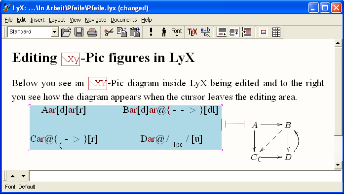
The following diagram, which is taken from the documentation of XY -Pic[1] by its creator Kristoffer H. Rose, will provide an example for many of the features available with that package. Its source code is:
Again, to turn this code into a graphical output, select it all at once starting from the \xymatrix{ ... up to the closing brace ... } and turn it into display-math as explained above. A moment after the cursor leaves the math-area, you should see the diagram in its full graphical glory as shown below.
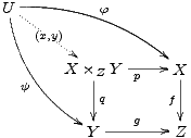
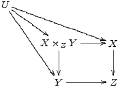
xymatrix uses a matrix to define the layout of the vertices of a diagram. For the above example, we need a 3 × 3-matrix of which 5 entries are used for the vertices U, X ×ZY , X, Y , Z, the other positions remaining empty. In this case, the following matrix determines the layout:
The pattern should be familiar from LATEX: We see three rows, each row being terminated by the end-of-line-marker \\ . Each line consists of entries, separated by the ampersand &.
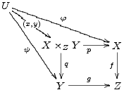
Having entered the vertices, we add arrows between them. The basic xypic-command to produce an arrow is \ar , it is entered into the cell of the matrix where the arrow is to start. The target of the arrow is defined by direction commands u (up) d (down) l (left), or r (right). These can be combined to a path and enclosed in square brackets. As an example, the arrows from the vertex U in the upper left corner down and right to the vertices X ×ZY , Y , and X are, respectively, defined as \ar[dr], \ar[ddr] and \ar[drr]. Thus the above diagram with all arrows added becomes:
Labels are attached to arrows by affixing them as upper or
lower indices to the \ar-command. Thus, \ar[drr]^\varphi defines an arrow going one cell down, two
to the right and having the label  attached
above. To attach a label below the arrow, make it a lower index as in \ar[ddr]_\psi. This explanation is correct only for arrows
pointing to the right. More precisely, imagine looking along the arrow in the
direction it is pointing. Then an upper index places a label to the left and a
lower index places it to the right. Consequently, an arrow pointing from right
to left, such as \ar[l]^\alpha_\beta will have label
attached
above. To attach a label below the arrow, make it a lower index as in \ar[ddr]_\psi. This explanation is correct only for arrows
pointing to the right. More precisely, imagine looking along the arrow in the
direction it is pointing. Then an upper index places a label to the left and a
lower index places it to the right. Consequently, an arrow pointing from right
to left, such as \ar[l]^\alpha_\beta will have label
 below and label
  above the
arrow, i.e.
above the
arrow, i.e. 
Using the character | instead of ^ or _ , it is even possible to place the label right onto the arrow, obscuring part of its shaft.
Normally, a label is placed halfway between an arrow's start and target objects. In the first diagram, the central arrow starting in U has the label (x,y) in the middle of the arrow's shaft, rather than in the middle between the two objects it connects. This is achieved by prefixing the label with a minus sign, here: \ar[dr]|-{(x,y)}.
Modification of the design, the form or the positioning of arrows are introduced by the @-character. This is followed by a pair of matching brackets, where the form of the bracket pair, { } or < > or / / indicates, whether we want to modify the design, the shift or the curvature of the arrow. Various modifactions can be applied to an arrow at the same time.
Various designs such as solid,
dotted, dashed or double are possible for the shaft of an arrow. These can be
combined with various ends and various tips. In general, the design of an arrow
is described by following the command \ar immediately
by an @-sign and a pair of braces {...} containg
characters describing the end, the shaft and the tip of the arrow. These
characters are chosen to give some form of ASCII-rendering of the real thing.
For instance \ar@{>..>>} produces an arow
with split end, a dotted shaft and double head. A number of other arrow designs
is given in the table below. Note that the ends of embedding arrows  are described by
raising or lowering opening parentheses, such as in \ar@{^(->}[r].
are described by
raising or lowering opening parentheses, such as in \ar@{^(->}[r].
|
|
|
| Result | Source code in LY X |
|
|
|
 |
\ar |
|
|
|
 |
\ar@{-->} |
|
|
|
 |
\ar@{..>} |
|
|
|
 |
\ar@{~>} |
|
|
|
 |
\ar@{->>} |
|
|
|
 |
\ar@{-->>} |
|
|
|
 |
\ar@{>->>} |
|
|
|
 |
\ar@{_(->} |
|
|
|
 |
\ar@{^(->} |
|
|
|
 |
\ar@{|-|} |
|
|
|
Following the @-character by either a 2, 3, _,or a ^, we can
produce arrows with double, triple shaft or arrows showing only the lower or
upper half of their tips and ends. Arrows need not have tips nor ends, as the
last example shows :
|
|
|
| Result | Source code for LY X |
|
|
|
 |
\ar@2 |
|
|
|
 |
\ar@3 |
|
|
|
 |
\ar@_{->} |
|
|
|
 |
\ar@^{->} |
|
|
|
 |
\ar@^{>>->>} |
|
|
|
 |
\ar@{^<-_>} |
|
|
|
 |
\ar@2{--} |
|
|
|
Arrows are shifted sideways with the modifier @<... > where the ellipsis is replaced by a positive or negative measure. For instance, to design a pair of mutually opposing arrows between two nodes, we shift them to see them apart. Note that the direction of the shift (positive) is to the left if one looks along the arrow. Thus
\[\xymatrix{\circ \ar@<1ex>[r]& \circ \ar@<1ex>[l]}\]
produces

Arrows and diagrams can be used inline, as this one:  . For this they
should be placed inside an inline math-environment $ ...$ or \(...\). To center a
diagram put it inside display-math patrrentheses \[
and \]. Diagrams constructed inline can later
be centered, or, conversely, centered diagrams can be changed to inline formuls
with Edit Math Alignment.
. For this they
should be placed inside an inline math-environment $ ...$ or \(...\). To center a
diagram put it inside display-math patrrentheses \[
and \]. Diagrams constructed inline can later
be centered, or, conversely, centered diagrams can be changed to inline formuls
with Edit Math Alignment.
There are two simple methods making arrows bend. The one is by giving an explicit value by which the midpoint of the arrow's shaft is raised or depressed, the other is by forcing the arrow to leave its origin in a prescribed compass direction and to make him enter the target at another direction. The necessary bending of the arrow is determined automatically. We describe both methods.
For bending arrows we use the modifier @/.../ . The ellipsis stands for a TEX-measure which needs to be entered as a lower or upper index. Whereas in xypic, we could simply write, e.g. \ar@/_1pc/ for an arrow bending 1pc downwards, this cannot directly be done in LY X. It is necessary, to provide an empty object {}, relative to which the index is placed, and the measure must be enclosed in braces, such as e.g. \ar@/{}_{1pc}/. As an example, here are two opposing arrows between A and B, each bending by .5 pica, given by the following source code:
\[\xymatrix{A \ar@/{}_{.5pc}/[r] & B \ar@/{}_{.5pc}/[l]}\]

An alternative for making arrows bend is by specifying their compass direction as they are leaving their source and their direction from which they enter their target. Instead of north, north-east, east, etc., the directions are named u, ur, r, dr, d, dl, l, ul, standing for up, up-right, right, down-right, etc.. A direction is specified as @(out,in) where out stands for the direction the first object is left and in stands for the direction from which the target is entered. As an example, we show some bending arrows and a loop, which arises when we do not specify a target for an arrow, just its incoming and outgoing direction:
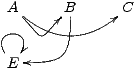
The above example is reminiscent of an automata diagram, except that in such a diagram states would be shown inside small circles, with double circles denoting final states.
With XY -Pic, entries can obtain a single or a double frame,
such as  or
or  by
prefixing an entry with *[F-] or *[F=] and enclosing the portion of the entry to be framed
in braces. Normally, the frame will be very tight so that it must be widened by
prefixing with + or with ++. Round frames, such as
by
prefixing an entry with *[F-] or *[F=] and enclosing the portion of the entry to be framed
in braces. Normally, the frame will be very tight so that it must be widened by
prefixing with + or with ++. Round frames, such as  and
and  are obtained by specifying the
shape as [o]. So the latter figure was constructed as
*++[o][F=]{B}. This way, the following automaton
are obtained by specifying the
shape as [o]. So the latter figure was constructed as
*++[o][F=]{B}. This way, the following automaton
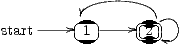
can be typeset as
& *++[o][F]{1}\ar[r]
& *++[o][F=]{2}\ar@(ur,dr)\ar@(ur,ul)[l]
}\].
The LATEX command \entrymodifiers={...} will make a certain entrystyle the default, that can, of course be overridden for individual entries. Thus, after \entrymodifiers={++[o][F-]}, all following entries inside XY -matrices would be encircled.
As an alternative to writing the xypic code, then transforming it into a math-editing environment by marking it and applying C-m, or C-M, one may construct and modify the whole xypic-diagram inside LY X's math editor. We describe the editing steps for a figure just like the one above.
Math
Add
Column, resp. M-m c i.
It is often convenient to stretch the horizontal or vertical dimension of a digram by using sacing commands for rows and columms. E.g. \xymatrix@R=1pc{...} defines an XY-matrix with row spacing of 1 pica. Unfortunately, this does currently not work inside LY X, since the @-character is interpreted by LY X as ending the XY-matrix-macro.
[1] Kristoffer H. Rose: XY -Pic User's Guide. Version 3.7, Feb. 16, 1999. Available as part of the xypic LATEX package.
[2] http://www.tug.org/tex-archive/help/Catalogue/entries/preview-latex.html
[3] http://www.tug.org/tex-archive/help/Catalogue/entries/xypic.html