Graphics Programming
3D Transformations
Thorsten Thormählen
November 04, 2022
Part 5, Chapter 2
Thorsten Thormählen
November 04, 2022
Part 5, Chapter 2
This is the print version of the slides.
Advance slides with the → key or
by clicking on the right border of the slide
Slides can also be advanced by clicking on the left or right border of the slide.
| Type | Font | Examples |
|---|---|---|
| Variables (scalars) | italics | $a, b, x, y$ |
| Functions | upright | $\mathrm{f}, \mathrm{g}(x), \mathrm{max}(x)$ |
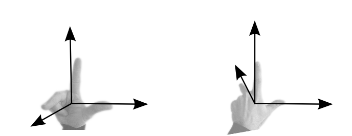
| Vectors | bold, elements row-wise | $\mathbf{a}, \mathbf{b}= \begin{pmatrix}x\\y\end{pmatrix} = (x, y)^\top,$ $\mathbf{B}=(x, y, z)^\top$ |
| Matrices | Typewriter | $\mathtt{A}, \mathtt{B}= \begin{bmatrix}a & b\\c & d\end{bmatrix}$ |
| Sets | calligraphic | $\mathcal{A}, B=\{a, b\}, b \in \mathcal{B}$ |
| Number systems, Coordinate spaces | double-struck | $\mathbb{N}, \mathbb{Z}, \mathbb{R}^2, \mathbb{R}^3$ |
GLfloat T[16];
GL_MODELVIEW matrix is responsible for the transformation of objects.glMatrixMode(GL_MODELVIEW);
glLoadIdentity, glLoadMatrix, glMultMatrix
glRotate, glScale, glTranslate, glPushMatrix, glPopMatrix
are then executed on the GL_MODELVIEW matrix.
GL_MODELVIEW matrix influences the transformation of objects only if they are drawn (OpenGL as a state machine)glLoadIdentity function sets the current GL_MODELVIEW matrix to a $4 \times 4$ identity matrix:
glMultMatrix, glRotate, glScale, glTranslate, create internally a $4 \times 4$ matrix that
is multiplied from the right to the current GL_MODELVIEW matrix
Example:
glMatrixMode(GL_MODELVIEW);
glLoadIdentity();
glTranslatef(...);
glRotatef(...);
glScalef(..);
$\mathtt{T}_{\mathrm{\small modelview}}= \mathtt{I}$
$\mathtt{T}_{\mathrm{\small modelview}}= \mathtt{I}\,\mathtt{T}_t$
$\mathtt{T}_{\mathrm{\small modelview}}= \mathtt{I}\,\mathtt{T}_t\,\mathtt{T}_r$
$\mathtt{T}_{\mathrm{\small modelview}}= \mathtt{I}\,\mathtt{T}_t\,\mathtt{T}_r\,\mathtt{T}_s $
$\underline{\tilde{\mathbf{P}}} = \mathtt{T}_{\mathrm{\small modelview}} \, \underline{\mathbf{P}}$
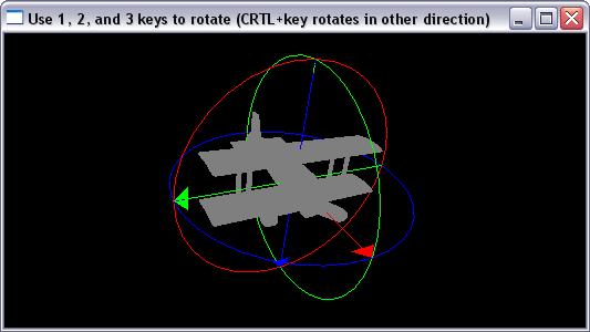
// rotate around z
glRotatef(rot1, 0.0, 0.0, 1.0);
// rotate around y
glRotatef(rot2, 0.0, 1.0, 0.0);
// rotate around x
glRotatef(rot3, 1.0, 0.0, 0.0);
class Renderer {
public:
float rot1;
float rot2;
float rot3;
public:
Renderer() : rot1(0.0), rot2(0.0), rot3(0.0) {}
public:
void display() {
glClearColor(0.0f, 0.0f, 0.0f, 0.0f);
glClear(GL_COLOR_BUFFER_BIT | GL_DEPTH_BUFFER_BIT);
glMatrixMode(GL_MODELVIEW);
glLoadIdentity();
// view scene from the side
glTranslatef(0.0,0.0,-3.0);
glRotatef( -45.0f, 0.0, 0.0, 1.0);
glRotatef( -45.0f, 0.0, 1.0, 0.0);
glRotatef( 135.0f, 1.0, 0.0, 0.0);
// rotate around z
glRotatef(rot1, 0.0, 0.0, 1.0);
glColor3f(0.0f, 0.0f, 1.0f);
drawCoordinateAxisZ();
// rotate around local y
glRotatef(rot2, 0.0, 1.0, 0.0);
glColor3f(0.0f, 1.0f, 0.0f);
drawCoordinateAxisY();
// rotate around local x
glRotatef(rot3, 1.0, 0.0, 0.0);
glColor3f(1.0f, 0.0f, 0.0f);
drawCoordinateAxisX();
// draw the plane in the local coordinate system
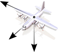
drawToyPlane();
}
private:
void drawCoordinateAxisZ() {
glBegin(GL_LINE_LOOP); // circle in x-y plane
for(int a=0; a<360; a+=10) {
float angle = M_PI / 180.0f * a;
glVertex3f(cos(angle), sin(angle), 0.0);
}
glEnd();
glBegin(GL_LINES);
glVertex3f(0.9f, 0.0f, 0.0f); // x-axis
glVertex3f(1.0f, 0.0f, 0.0f);
glVertex3f(0.0f, 0.9f, 0.0f); // y-axis
glVertex3f(0.0f, 1.0f, 0.0f);
glVertex3f(0.0f, 0.0f,-1.0f); // z-axis
glVertex3f(0.0f, 0.0f, 1.0f);
glEnd();
glBegin(GL_TRIANGLES); // z-axis tip
glVertex3f(0.0f,-0.1f, 0.9f);
glVertex3f(0.0f, 0.0f, 1.0f);
glVertex3f(0.0f, 0.1f, 0.9f);
glEnd();
}
void drawCoordinateAxisX() {
glPushMatrix();
glRotatef(90.0f, 0.0f, 1.0f, 0.0f);
drawCoordinateAxisZ();
glPopMatrix();
}
void drawCoordinateAxisY() {
glPushMatrix();
glRotatef(-90.0f, 1.0f, 0.0f, 0.0f);
drawCoordinateAxisZ();
glPopMatrix();
}
...
};
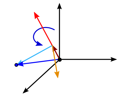
with $\mathbf{v}_n = (\mathbf{v}^\top \mathbf{n})\, \mathbf{n}$ it holds $\tilde{\mathbf{v}} = \mathbf{v}_n + (\mathbf{v} - \mathbf{v}_n) \cos \alpha + (\mathbf{n} \times \mathbf{v}) \sin \alpha$
with $\mathbf{v}_n = (\mathbf{v}^\top \mathbf{n})\, \mathbf{n} = (\mathbf{n}^\top \mathbf{v} )\, \mathbf{n} = (\mathbf{n} \mathbf{n}^\top) \mathbf{v}$ we have:
$\begin{align} \tilde{\mathbf{v}} &= \mathbf{v}_n + (\mathbf{v} - \mathbf{v}_n) \cos \alpha + (\mathbf{n} \times \mathbf{v}) \sin \alpha\\ \tilde{\mathbf{v}} &= (\mathbf{n} \mathbf{n}^\top) \mathbf{v} + (\mathbf{v} - (\mathbf{n}\mathbf{n}^\top ) \mathbf{v}) \cos \alpha + ([\mathbf{n}]_\times \mathbf{v}) \sin \alpha\\ \tilde{\mathbf{v}} &= \mathtt{R} \mathbf{v} \end{align}$
the resulting $3 \times 3$ rotation matrix is a function of $\mathbf{n}$ and $\alpha$, which can be calculated by
$ \mathtt{R} = (\mathbf{n} \mathbf{n}^\top) + (\cos \alpha) (\mathbf{I}_{3\times 3} - (\mathbf{n} \mathbf{n}^\top)) + (\sin \alpha)
[\mathbf{n}]_\times$
Thus, the rotation matrix has 4 degrees of freedom $\mathbf{n}=(n_x, n_y, n_z)$ and $\alpha$. Or more exactly, because $|\mathbf{n}|=1$, there are really only 3 degrees of freedom (equivalent to the representation using Euler angles)
$\mathbf{q} = \begin{pmatrix}q_1\\q_2\\ q_3\\ q_4\end{pmatrix} = \begin{pmatrix}s \\v_x \\ v_y \\ v_z\end{pmatrix} = (s, \mathbf{v}^\top)^\top$
Quaternion fastmul(Quaternion ql, Quaternion qr) {
double s[9], t;
s[0] = (ql.vz-ql.vy)*(qr.vy-qr.vz); s[1] = (ql.s +ql.vx)*(qr.s +qr.vx);
s[2] = (ql.s -ql.vx)*(qr.vy+qr.vz); s[3] = (ql.vz+ql.vy)*(qr.s -qr.vx);
s[4] = (ql.vz-ql.vx)*(qr.vx-qr.vy); s[5] = (ql.vz+ql.vx)*(qr.vx+qr.vy);
s[6] = (ql.s +ql.vy)*(qr.s -qr.vz); s[7] = (ql.s -ql.vy)*(qr.s +qr.vz);
s[8] = s[5]+s[6]+s[7];
t = (s[4]+s[8])*0.5;
return Quaternion(s[0]+t-s[5], s[1]+t-s[8], s[2]+t-s[7], s[3]+t-s[6]);
}
class Renderer {
public:
Renderer() : t(0.0) {}
public:
void display() {
glClearColor(0.0f, 0.0f, 0.0f, 0.0f);
glClear(GL_COLOR_BUFFER_BIT | GL_DEPTH_BUFFER_BIT);
glMatrixMode(GL_MODELVIEW);
glLoadIdentity();
// view scene from the side
glTranslatef(0.0,0.0,-3.0);
glRotatef( -45.0f, 0.0, 0.0, 1.0);
glRotatef( -45.0f, 0.0, 1.0, 0.0);
glRotatef( 135.0f, 1.0, 0.0, 0.0);
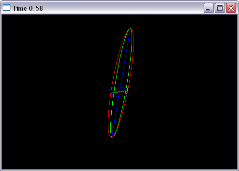
if(true) {
// interpolate rotation matrices, which is wrong
float r0[16];
float r1[16];
float rt[16];
glPushMatrix(); // save for later use
glLoadIdentity();
glGetFloatv(GL_MODELVIEW_MATRIX, r0);
glRotatef(180.0f, 0.0, 0.0, 1.0); // rotate around z
glGetFloatv(GL_MODELVIEW_MATRIX, r1);
glPopMatrix(); // restore
for(unsigned i=0; i < 16; i++) {
rt[i] = (1-t) * r0[i] + t * r1[i]; //interpolate
}
glMultMatrixf(rt); // apply matrix
}else{
// interpolate rotation angle, which is correct
glRotatef(t*180.0f, 0.0, 0.0, 1.0); // rotate around z
}
glColor3f(0.0f, 0.0f, 1.0f);
drawCoordinateAxisZ();
glColor3f(0.0f, 1.0f, 0.0f);
drawCoordinateAxisY();
glColor3f(1.0f, 0.0f, 0.0f);
drawCoordinateAxisX();
}
...
};
Please notify me by e-mail if you have questions, suggestions for improvement, or found typos: Contact