Grafikprogrammierung
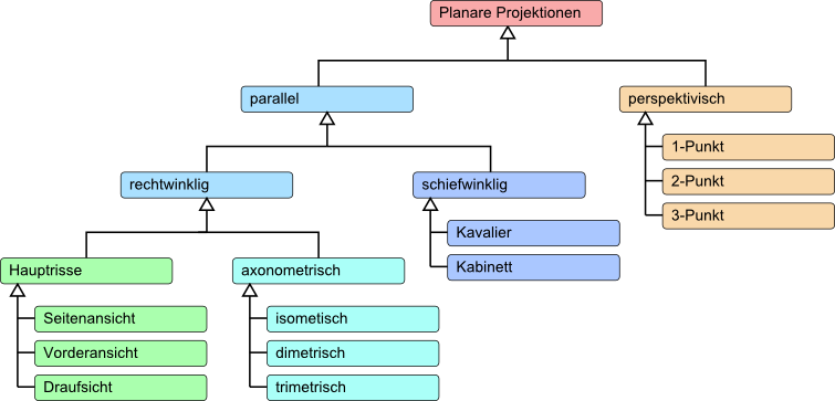
Kameras: Parallelprojektion
Thorsten Thormählen
22. November 2024
Teil 6, Kapitel 2
Thorsten Thormählen
22. November 2024
Teil 6, Kapitel 2
Dies ist die Druck-Ansicht.
Weiterschalten der Folien durch die → Taste oder
durch das Klicken auf den rechten Folienrand.
Das Weiterschalten der Folien kann ebenfalls durch das Klicken auf den rechten bzw. linken Folienrand erfolgen.
| Typ | Schriftart | Beispiele |
|---|---|---|
| Variablen (Skalare) | kursiv | $a, b, x, y$ |
| Funktionen | aufrecht | $\mathrm{f}, \mathrm{g}(x), \mathrm{max}(x)$ |
| Vektoren | fett, Elemente zeilenweise | $\mathbf{a}, \mathbf{b}= \begin{pmatrix}x\\y\end{pmatrix} = (x, y)^\top,$ $\mathbf{B}=(x, y, z)^\top$ |
| Matrizen | Schreibmaschine | $\mathtt{A}, \mathtt{B}= \begin{bmatrix}a & b\\c & d\end{bmatrix}$ |
| Mengen | kalligrafisch | $\mathcal{A}, B=\{a, b\}, b \in \mathcal{B}$ |
| Zahlenbereiche, Koordinatenräume | doppelt gestrichen | $\mathbb{N}, \mathbb{Z}, \mathbb{R}^2, \mathbb{R}^3$ |

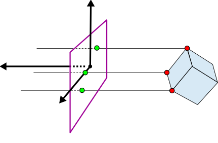
$\tilde{\mathbf{P}}= \left(p_x, p_y, 0 \right)^\top$
$\begin{align}\underline{\tilde{\mathbf{P}}} & = \begin{pmatrix}p_x \\ p_y \\ 0\\ 1\end{pmatrix} = \underbrace{\begin{bmatrix} 1 & 0 & 0 & 0 \\ 0 & 1 & 0 & 0 \\ 0 & 0 & 0 & 0 \\ 0 & 0 & 0 & 1 \end{bmatrix}}_{\mathtt{A}} \begin{pmatrix}p_x \\p_y \\ p_z\\ 1\end{pmatrix}\\ \underline{\tilde{\mathbf{P}}} &=\mathtt{A}\, \underline{\mathbf{P}} \end{align}$
$\mathtt{A} = \begin{bmatrix} \alpha_x & 0 & 0 & \beta_x \\ 0 & \alpha_y & 0 & \beta_y \\ 0 & 0 & -\alpha_z & \beta_z \\ 0 & 0 & 0 & 1 \end{bmatrix}$
$\underline{\tilde{\mathbf{P}}} = \begin{pmatrix}\alpha_x \, p_x + \beta_x \\ \alpha_y \, p_y + \beta_y \\ -\alpha_z \, p_z + \beta_z \\ 1\end{pmatrix} = \begin{bmatrix} \alpha_x & 0 & 0 & \beta_x \\ 0 & \alpha_y & 0 & \beta_y \\ 0 & 0 & -\alpha_z & \beta_z \\ 0 & 0 & 0 & 1 \end{bmatrix} \begin{pmatrix}p_x \\p_y \\ p_z\\ 1\end{pmatrix} \in \mathbb{H}^3$
$\begin{align} \alpha_z &= \frac{2}{z_f-z_n}\\ \beta_z & = -\frac{z_f + z_n}{z_f-z_n}\end{align}$
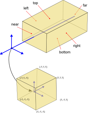
$\mathtt{A} = \begin{bmatrix} \frac{2}{x_r-x_l} & 0 & 0 & -\frac{x_r + x_l}{x_r-x_l} \\ 0 & \frac{2}{y_t-y_b} & 0 & -\frac{y_t + y_b}{y_t-y_b} \\ 0 & 0 & \frac{-2}{z_f-z_n} & -\frac{z_f + z_n}{z_f-z_n} \\ 0 & 0 & 0 & 1 \end{bmatrix}$
Erzeugen einer $4 \times 4$ Parallelprojektionsmatrix in OpenGL:
glMatrixMode(GL_PROJECTION);
glLoadIdentity();
glOrtho(left, right, bottom, top, near, far);
$\mathtt{A} = \begin{bmatrix} \frac{2}{\mathrm{right}-\mathrm{left}} & 0 & 0 & -\frac{\mathrm{right} + \mathrm{left}}{\mathrm{right}-\mathrm{left}} \\ 0 & \frac{2}{\mathrm{top}-\mathrm{bottom}} & 0 & -\frac{\mathrm{top} + \mathrm{bottom}}{\mathrm{top}-\mathrm{bottom}} \\ 0 & 0 & \frac{-2}{\mathrm{far}-\mathrm{near}} & -\frac{\mathrm{far} + \mathrm{near}}{\mathrm{far}-\mathrm{near}} \\ 0 & 0 & 0 & 1 \end{bmatrix}$
$\mathtt{A} \mathtt{T}_{\mathrm{\small cam}}^{-1} = \mathtt{A} \, \mathtt{T}_R(90^\circ)$
$\mathtt{A} \mathtt{T}_{\mathrm{\small cam}}^{-1} = \mathtt{A} \, \mathtt{T}_r(\mathbf{n}, \alpha)$
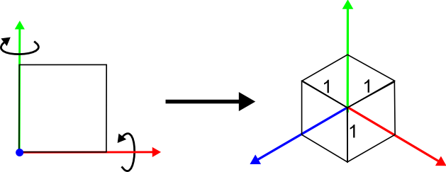
$\begin{align} \mathtt{A} \mathtt{T}_{\mathrm{\small cam}}^{-1} & = \mathtt{A} \, \mathtt{T}_{r_x}(\beta) \, \mathtt{T}_{r_y}(\alpha)\\ & = \begin{bmatrix} 1 & 0 & 0 & 0 \\ 0 & 1 & 0 & 0 \\ 0 & 0 & 0 & 0 \\ 0 & 0 & 0 & 1 \end{bmatrix} \begin{bmatrix} 1 & 0 & 0 & 0 \\ 0& \cos \beta & -\sin \beta& 0 \\ 0 & \sin \beta & \cos \beta & 0 \\ 0 & 0 & 0 &1 \\ \end{bmatrix} \begin{bmatrix} \cos \alpha & 0& \sin \alpha& 0 \\ 0 & 1 & 0 & 0 \\ -\sin \alpha & 0 &\cos \alpha & 0 \\ 0 & 0 & 0 &1 \\ \end{bmatrix} \\ & = \begin{bmatrix} 1 & 0 & 0 & 0 \\ 0 & 1 & 0 & 0 \\ 0 & 0 & 0 & 0 \\ 0 & 0 & 0 & 1 \end{bmatrix} \begin{bmatrix} \cos \alpha & 0 & \sin \alpha & 0 \\ \sin \beta \sin \alpha & \cos \beta & -\sin \beta \cos \alpha & 0\\ - \cos \beta \sin \alpha & \sin \beta & \cos \beta \cos \alpha & 0 \\ 0 & 0 & 0 & 1 \\ \end{bmatrix} \\ & = \begin{bmatrix} \cos \alpha & 0 & \sin \alpha & 0 \\ \sin \beta \sin \alpha & \cos \beta & -\sin \beta \cos \alpha & 0\\ 0 & 0 & 0 & 0 \\ 0 & 0 & 0 & 1 \\ \end{bmatrix} \end{align}$
$ \underline{\tilde{\mathbf{e}}}_x = \begin{pmatrix}\cos \alpha\\ \sin \beta \sin \alpha \\ 0\\ 1\\ \end{pmatrix}, \quad \underline{\tilde{\mathbf{e}}}_y = \begin{pmatrix}0\\ \cos \beta \\ 0\\ 1\\ \end{pmatrix}, \quad \underline{\tilde{\mathbf{e}}}_z = \begin{pmatrix}\sin \alpha\\ -\sin \beta \cos \alpha \\ 0\\ 1\\ \end{pmatrix}$
$\begin{align} |\tilde{\mathbf{e}}_x| &= \sqrt{\cos^2\alpha + (\sin \beta \sin \alpha)^2}\\ |\tilde{\mathbf{e}}_y| &= \sqrt{\cos^2\beta}\\ |\tilde{\mathbf{e}}_z| &= \sqrt{\sin^2\alpha + (\sin \beta \cos \alpha)^2}\\ \end{align}$
class Renderer {
public:
int mode;
private:
double alpha;
double beta;
public:
Renderer() : mode(1), alpha(0.0), beta(0.0) {}
public:
void display() {
glClearColor(1.0f, 1.0f, 1.0f, 0.0f);
glClear(GL_COLOR_BUFFER_BIT | GL_DEPTH_BUFFER_BIT);
glMatrixMode(GL_MODELVIEW);
glLoadIdentity();
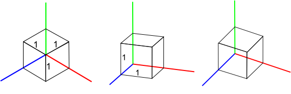
if(mode == 1) { // isometric
alpha = 45.0;
beta = 180.0 / M_PI * atan(1.0/sqrt(2.0));
}
if(mode == 2) { // dimetric
alpha= 180.0 / M_PI * atan(1.0/sqrt(7.0));
beta = 180.0 / M_PI * atan(1.0/(2.0*sqrt(2.0)));
}
if(mode == 3) { // trimetric
alpha= 30.0;
beta = 35.0;
}
if(mode < 4) {
glRotatef( beta, 1.0, 0.0f, 0.0);
glRotatef(-alpha, 0.0f, 1.0f, 0.0f);
}
if(mode == 4) { // isometric
//alternativ implementation
gluLookAt(1.0, 1.0, 1.0, // eye
0.0, 0.0, 0.0, // look at
0.0, 1.0, 0.0); //up
}
if(mode == 5) { // dimetric
//alternativ implementation
gluLookAt(1.0, 1.0, sqrt(7.0),
0.0, 0.0, 0.0,
0.0, 1.0, 0.0);
}
glColor3f(0.0f, 0.0f, 1.0f);
drawCoordinateAxisZ();
glColor3f(0.0f, 1.0f, 0.0f);
drawCoordinateAxisY();
glColor3f(1.0f, 0.0f, 0.0f);
drawCoordinateAxisX();
drawUnitCube();
}
void init() {
glEnable(GL_DEPTH_TEST);
}
void resize(int w, int h) {
double aspect = float(w)/float(h);
glViewport(0, 0, w, h);
glMatrixMode(GL_PROJECTION);
glLoadIdentity();
glOrtho(-2.0*aspect, 2.0*aspect, -2.0, 2.0, -5.0, 5.0);
}
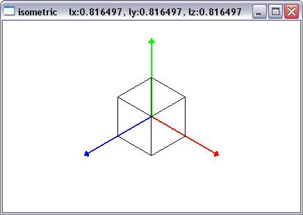
void getAbsLengthXYZ(float& lx, float& ly, float &lz) {
double cb = cos(beta/180.0*M_PI);
double ca = cos(alpha/180.0*M_PI);
double sb = sin(beta/180.0*M_PI);
double sa = sin(alpha/180.0*M_PI);
lx = sqrt(ca*ca+sb*sb*sa*sa);
ly = sqrt(cb*cb);
lz = sqrt(sa*sa+sb*sb*ca*ca);
}
...
};
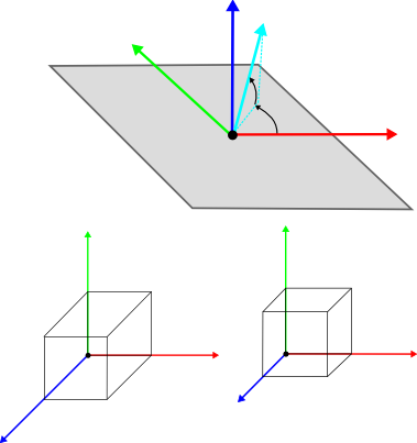
$\mathtt{A} \mathtt{T}_{\mathrm{\small cam}}^{-1} = \begin{bmatrix} 1 & 0 & 0 & 0 \\ 0 & 1 & 0 & 0 \\ 0 & 0 & 0 & 0 \\ 0 & 0 & 0 & 1 \end{bmatrix} \begin{bmatrix} 1 & 0 & \frac{-\cos \alpha}{\tan \beta} & 0 \\ 0 & 1 & \frac{\sin \alpha}{\tan \beta} & 0 \\ 0 & 0 & \frac{-1}{\sin \beta} & 0 \\ 0 & 0 & 0 & 1 \end{bmatrix} =\begin{bmatrix} 1 & 0 & \frac{-\cos \alpha}{\tan \beta} & 0 \\ 0 & 1 & \frac{\sin \alpha}{\tan \beta} & 0 \\ 0 & 0 & 0 & 0 \\ 0 & 0 & 0 & 1 \end{bmatrix}$
$\mathtt{A} \mathtt{T}_{\mathrm{\small cam}}^{-1} = \begin{bmatrix} 1 & 0 & -\cos \alpha & 0 \\ 0 & 1 & \sin \alpha & 0 \\ 0 & 0 & 0 & 0 \\ 0 & 0 & 0 & 1 \end{bmatrix}$
$\mathtt{A} \mathtt{T}_{\mathrm{\small cam}}^{-1} = \begin{bmatrix} 1 & 0 & \frac{-\cos \alpha}{2} & 0 \\ 0 & 1 & \frac{\sin \alpha}{2} & 0 \\ 0 & 0 & 0 & 0 \\ 0 & 0 & 0 & 1 \end{bmatrix}$
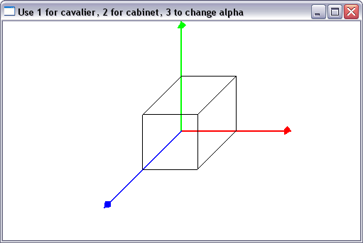
class Renderer {
public:
  int mode;
  double alpha;

public:
  Renderer() : mode(1), alpha(-45.0) {}

public:
  void display() {
    glClearColor(1.0f, 1.0f, 1.0f, 0.0f);
    glClear(GL_COLOR_BUFFER_BIT | GL_DEPTH_BUFFER_BIT);


    glMatrixMode(GL_MODELVIEW);
    glLoadIdentity();
    float m[16]; // identity
    glGetFloatv(GL_MODELVIEW_MATRIX, m);
    float angle = (M_PI / 180.0f) * alpha;
    if(mode == 1) { // cavalier
      m[2*4+0] = -cos(angle);
      m[2*4+1] = sin(angle);
    }
    if(mode == 2) { // cabinet
      m[2*4+0] = -cos(angle)/2.0f;
      m[2*4+1] = sin(angle)/2.0f;
    }
    glMultMatrixf(m);

    glColor3f(0.0f, 0.0f, 1.0f);
    drawCoordinateAxisZ();
    glColor3f(0.0f, 1.0f, 0.0f);
    drawCoordinateAxisY();
    glColor3f(1.0f, 0.0f, 0.0f);
    drawCoordinateAxisX();

    drawUnitCube();
  }

  void init() {
    glEnable(GL_DEPTH_TEST);
  }

  void resize(int w, int h) {
    double aspect = float(w)/float(h);
    glViewport(0, 0, w, h);
    glMatrixMode(GL_PROJECTION);
    glLoadIdentity();
    glOrtho(-2.0*aspect, 2.0*aspect, -2.0, 2.0, -5.0, 5.0);
  }
...
};
Anregungen oder Verbesserungsvorschläge können auch gerne per E-mail an mich gesendet werden: Kontakt