Graphics Programming
Light and Materials
Thorsten Thormählen
December 20, 2024
Part 10, Chapter 1
Thorsten Thormählen
December 20, 2024
Part 10, Chapter 1
This is the print version of the slides.
Advance slides with the → key or
by clicking on the right border of the slide
Slides can also be advanced by clicking on the left or right border of the slide.
| Type | Font | Examples |
|---|---|---|
| Variables (scalars) | italics | $a, b, x, y$ |
| Functions | upright | $\mathrm{f}, \mathrm{g}(x), \mathrm{max}(x)$ |
| Vectors | bold, elements row-wise | $\mathbf{a}, \mathbf{b}= \begin{pmatrix}x\\y\end{pmatrix} = (x, y)^\top,$ $\mathbf{B}=(x, y, z)^\top$ |
| Matrices | Typewriter | $\mathtt{A}, \mathtt{B}= \begin{bmatrix}a & b\\c & d\end{bmatrix}$ |
| Sets | calligraphic | $\mathcal{A}, B=\{a, b\}, b \in \mathcal{B}$ |
| Number systems, Coordinate spaces | double-struck | $\mathbb{N}, \mathbb{Z}, \mathbb{R}^2, \mathbb{R}^3$ |
| Symbol | Meaning |
|---|---|
| $\Omega$ | Solid angle |
| $\theta$ | Polar angle in the spherical coordinate system |
| $\phi$ | Azimuth angle in the spherical coordinate system |
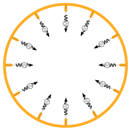
| $\Phi$ | Radiant flux |
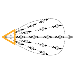
| $I$ | Radiant intensity |
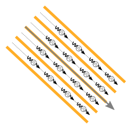
| $E$ | Irradiance |
| $L$ | Radiance |
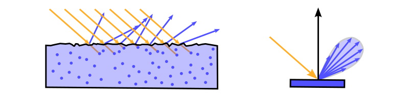
| $\mathrm{f}_r$ | BRDF (Bidirectional Reflection Distribution Function) |
| $\mathrm{f}_d$ | Diffuse part of the BRDF |
| $\mathrm{f}_s$ | Specular part of the BRDF |
| Symbol | Meaning |
|---|---|
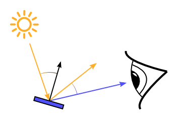
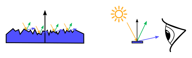
| $\mathbf{n}$ | Surface normal |
| $\mathbf{v}$ | Unit vector in view direction |
| $\mathbf{l}$ | Unit vector in light direction |
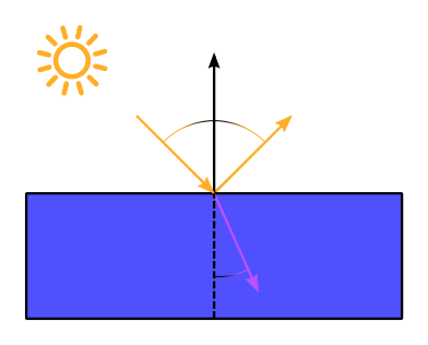
| $\eta$ | Refractive index |
| $F$ | Fresnel reflectance |
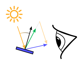
| $\mathbf{h}$ | Halfway vector between light and view direction |
| $(\dots)_+$ | Ramp function |
| $\langle \mathbf{a}\cdot \mathbf{b}\rangle$ | Scalar product |
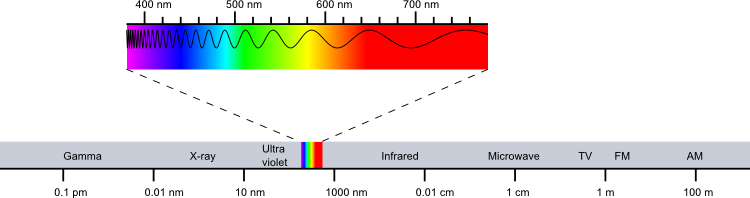
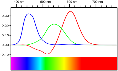
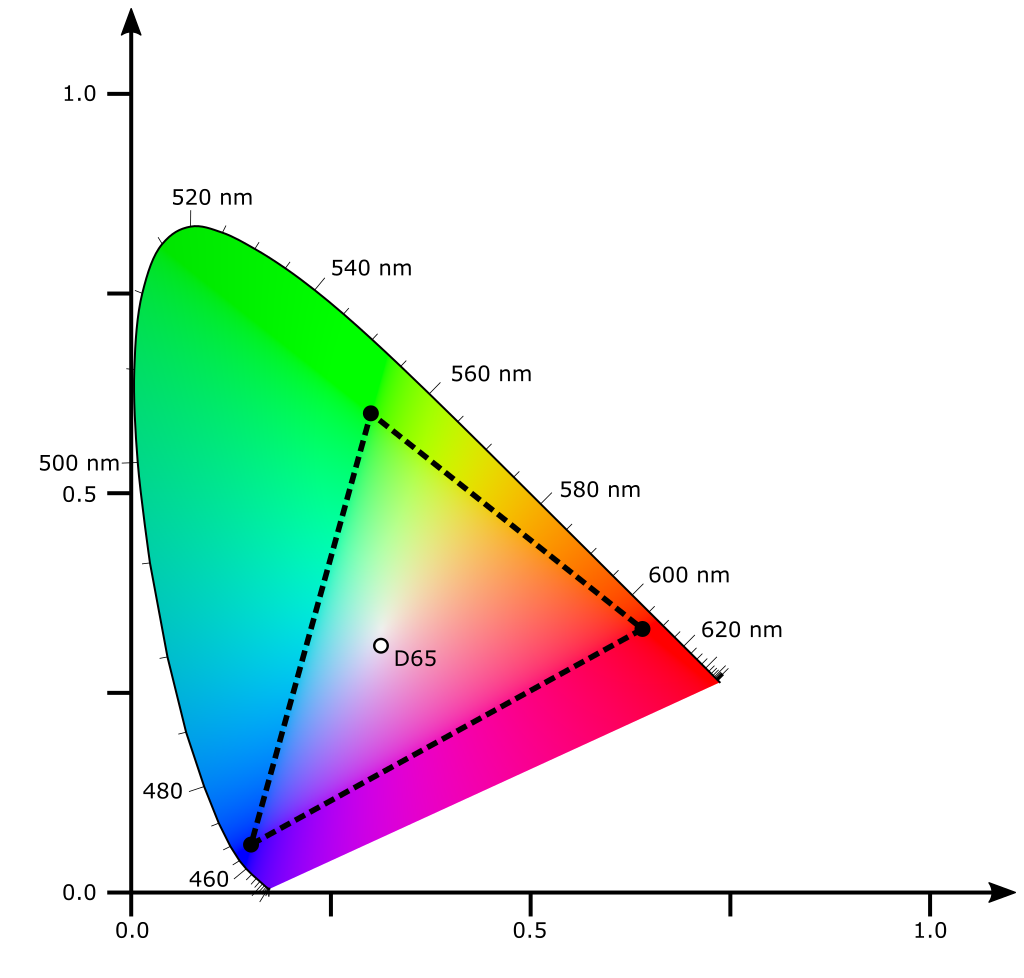
| $\lambda$ | Wavelength |
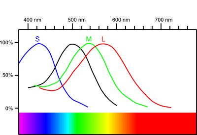
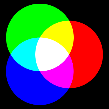
There are two systems of light sensory cells in humans:
| (red, green, blue) | Farbe |
|---|---|
| (1.0, 0.0, 0.0) | |
| (0.0, 1.0, 0.0) | |
| (0.0, 0.0, 1.0) | |
| (1.0, 1.0, 0.0) | |
| (1.0, 0.0, 1.0) | |
| (0.0, 1.0, 1.0) | |
| (0.0, 0.0, 0.0) | |
| (0.5, 0.5, 0.5) | |
| (1.0, 1.0, 1.0) | |
| (0.2, 0.4, 0.0) | |
| (0.8, 0.2, 0.3) |
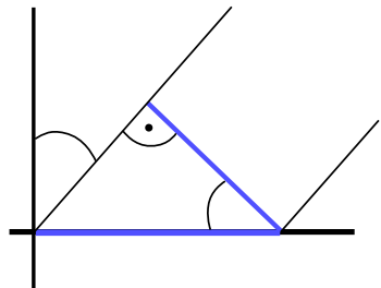
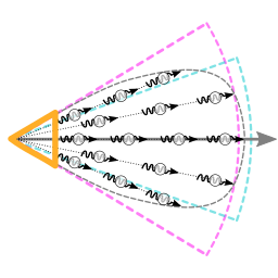
Angle in 2D Solid angle in 3D
$\alpha = \frac{s}{r}$ $\Omega = \frac{S}{r^2}$
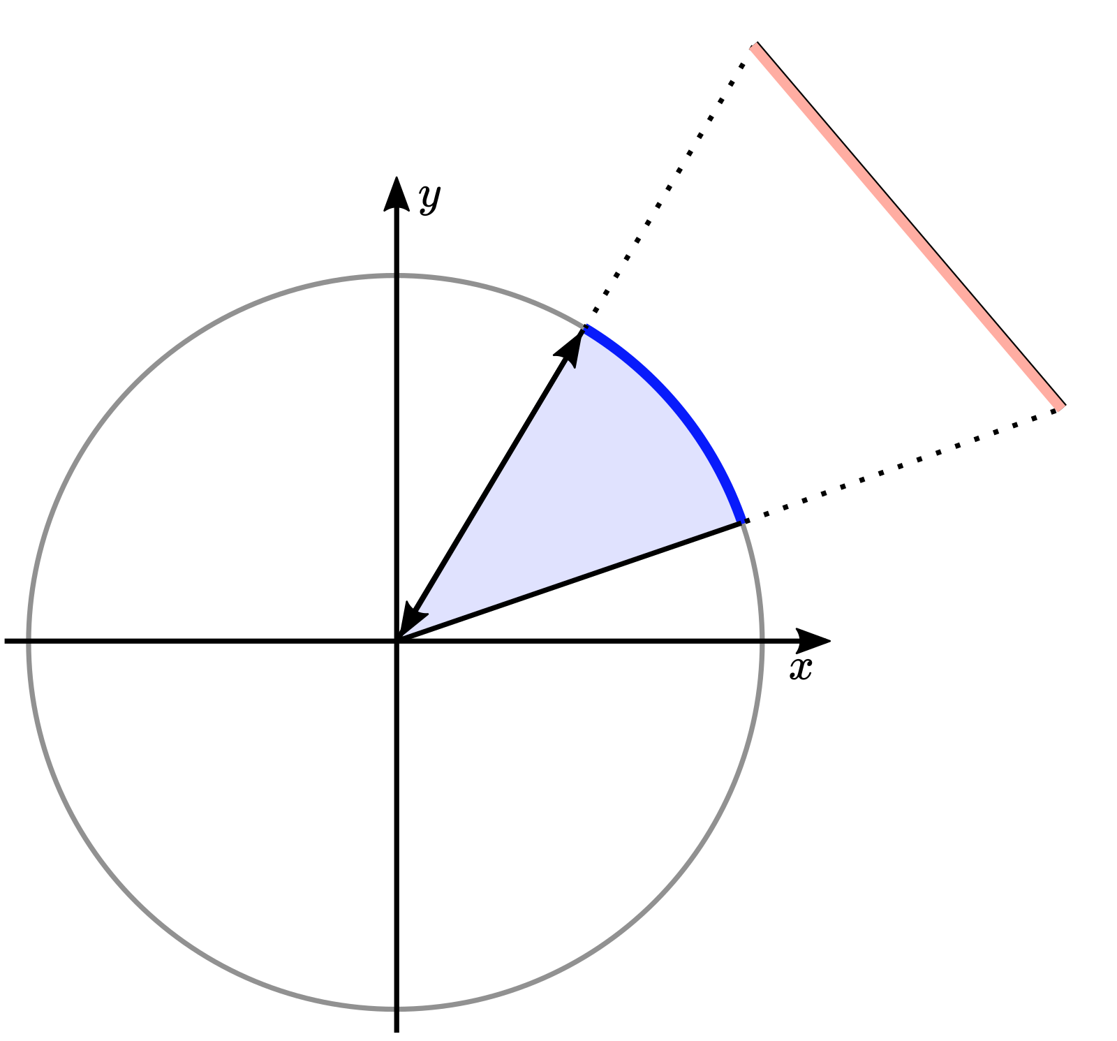
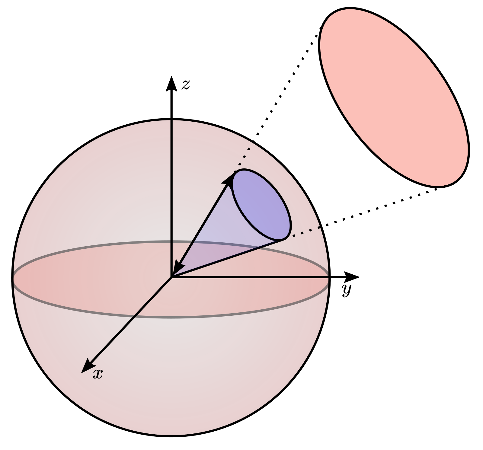
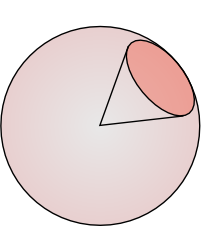
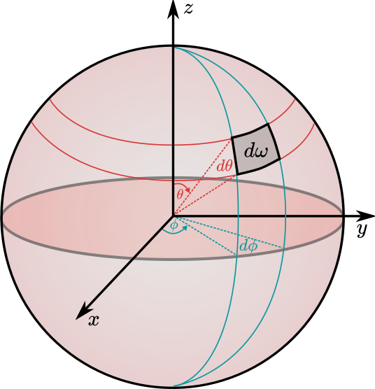
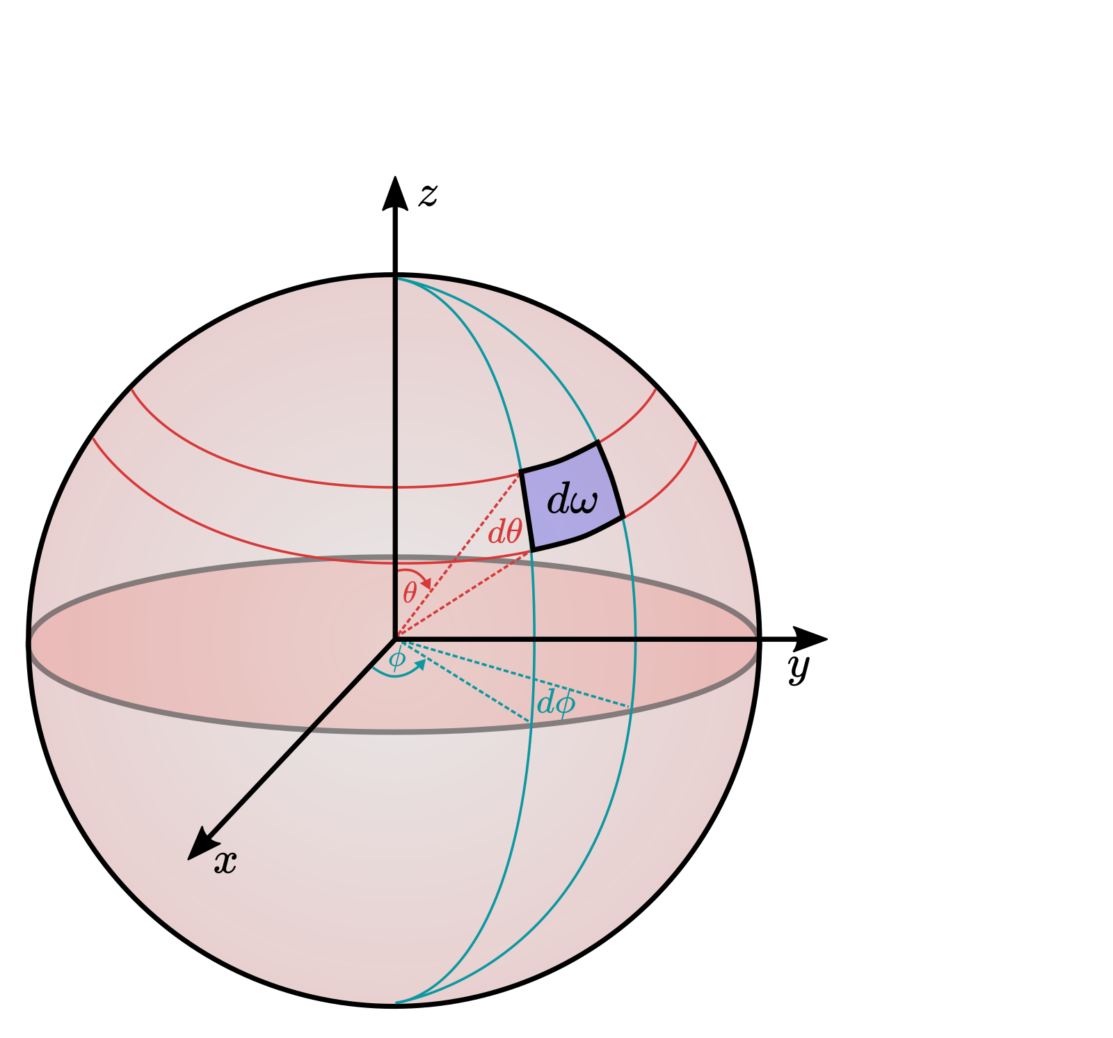
$\Omega = \int\limits_{\omega}d\omega = \frac{S}{r^2}$
$\Omega = \int\limits_{\omega}d\omega = \int\limits_{\omega}d\theta(\sin \theta \, d\phi)= \int\limits_{\phi}\int\limits_{\theta}\sin \theta \, d\theta \, d\phi$
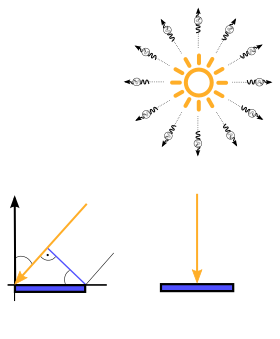
$\Phi = \frac{dQ}{dt} \approx \frac{\Delta Q}{\Delta t}$
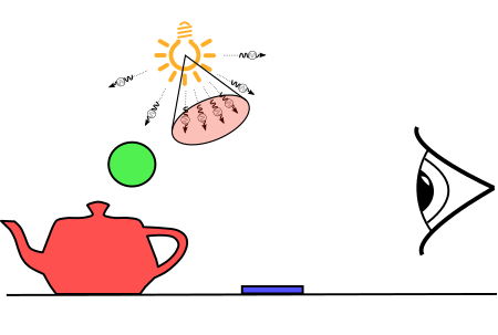
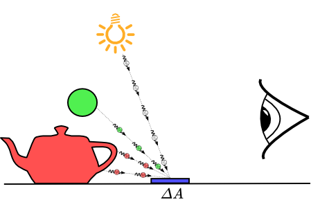
$E = \frac{d\Phi}{dA} \approx \frac{\Delta \Phi}{\Delta A}$
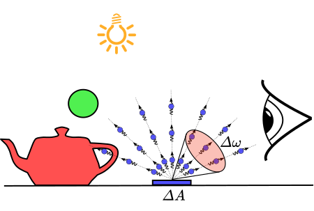
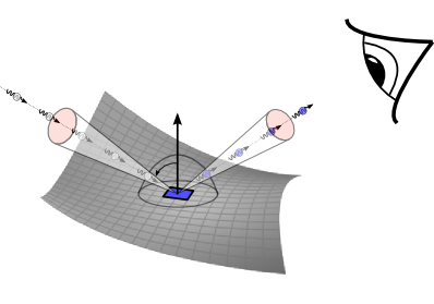
$L = \frac{d^2\Phi}{d\omega\, \cos(\theta) \,dA} \approx \frac{\Delta \Phi}{\Delta \omega\, \cos(\theta) \,\Delta A}$
$L_o(\mathbf{v}) = L_e(\mathbf{v}) + \int\limits_\Omega \mathrm{f}_r(\mathbf{v}, \mathbf{l})\, \, \underbrace{L_i(\mathbf{l}) \cos(\theta) \, d\omega}_{dE(\mathbf{l})}$
$\mathrm{f}_r(\mathbf{v}, \mathbf{l}) = \frac{ dL_o(\mathbf{v})} { dE(\mathbf{l})} $
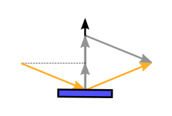
reflect to calculate the reflection direction $\mathbf{r}$
vec3 reflectDir = reflect(-lightDir, normal);
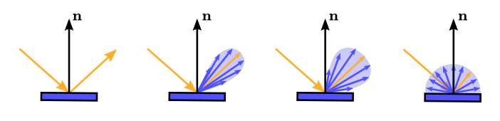
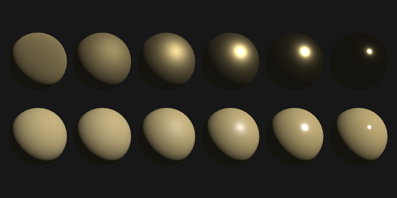
$\mathbf{l}$ $\mathbf{v}$ $k_d$ $k_s$ $n_s$
x = max(x, 0.0);
$\mathbf{l}$ $\mathbf{v}$ $k_d$ $k_s$ $n_s$


#version 140
in vec3 position;
in vec2 texcoord;
in vec3 normal;

uniform mat4 projection;
uniform mat4 modelview;
uniform mat4 normalMat;

out vec2 tc;
out vec3 fn;
out vec3 vertPos;

void main(){
  tc = texcoord;
  fn = vec3(normalMat * vec4(normal, 0.0));
  vec4 vertPos4 = modelview * vec4(position, 1.0);
  vertPos = vec3(vertPos4) / vertPos4.w;
  gl_Position = projection * modelview * vec4(position, 1.0);
}
#version 140
out vec4 outColor;
in vec2 tc;
in vec3 fn;
in vec3 vertPos;
uniform int mode;
uniform vec3 lightDirection;
const vec4 ambientColor = vec4(0.01, 0.0, 0.0, 1.0);
const vec4 diffuseColor = vec4(0.25, 0.0, 0.0, 1.0);
const vec4 specularColor = vec4(1.0, 1.0, 1.0, 1.0);
const float shininess = 20.0;
const vec4 lightColor = vec4(1.0, 1.0, 1.0, 1.0);
const float irradiPerp = 1.0;
vec3 phongBRDF(vec3 lightDir, vec3 viewDir, vec3 normal,
vec3 phongDiffuseCol, vec3 phongSpecularCol, float phongShininess) {
vec3 color = phongDiffuseCol;
vec3 reflectDir = reflect(-lightDir, normal);
float specDot = max(dot(reflectDir, viewDir), 0.0);
color += pow(specDot, phongShininess) * phongSpecularCol;
return color;
}
void main() {
vec3 lightDir = normalize(-lightDirection);
vec3 viewDir = normalize(-vertPos);
vec3 n = normalize(fn);
vec3 radiance = ambientColor.rgb;
float irradiance = max(dot(lightDir, n), 0.0) * irradiPerp;
if(irradiance > 0.0) {
vec3 brdf = phongBRDF(lightDir, viewDir, n,
diffuseColor.rgb, specularColor.rgb, shininess);
radiance += brdf * irradiance * lightColor.rgb;
}
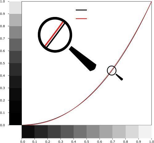
radiance = pow(radiance, vec3(1.0 / 2.2) ); // gamma correction
outColor.rgb = radiance;
outColor.a = 1.0;
}uniform variable
(as shown in the previous example)mat4 cameraProjection is the transformation $\mathtt{A}$ from the camera coordinate system into the image planemat4 cameraLookAt is the transformation $\mathtt{T}_{\mathrm{\small cam}}^{-1}$ from the world coordinate system to the camera coordinate systemmat4 meshTransform is the transformation $\mathtt{T}_{\mathrm{\small obj}}$ from the local coordinate system to the world coordinate systemmat4 meshTransformTransposedInverse is the transformation $\mathtt{T}_{\mathrm{\small obj}}^{-\top}$ of the normal into the world coordinate system
#version 140
in vec3 position;
in vec2 texcoord;
in vec3 normal;

uniform mat4 cameraLookAt;
uniform mat4 cameraProjection;
uniform mat4 meshTransform;
uniform mat4 meshTransformTransposedInverse;

out vec2 tc;
out vec3 wfn;
out vec3 vertPos;

void main(){
  tc = texcoord;
  wfn = vec3(meshTransformTransposedInverse * vec4(normal, 0.0));
  vec4 vertPos4 = meshTransform * vec4(position, 1.0);
  vertPos = vec3(vertPos4) / vertPos4.w;
  gl_Position = cameraProjection * cameraLookAt * vertPos4;
}
#version 140
out vec4 outColor;

in vec2 tc;
in vec3 wfn;
in vec3 vertPos;

uniform int mode;
uniform vec3 cameraPosition;

const vec3 lightDirection = vec3(0.0, -1.0, -1.0);
const vec4 ambientColor = vec4(0.01, 0.0, 0.0, 1.0);
const vec4 diffuseColor = vec4(0.25, 0.0, 0.0, 1.0);
const vec4 specularColor = vec4(1.0, 1.0, 1.0, 1.0);
const float shininess = 20.0;
const vec4 lightColor = vec4(1.0, 1.0, 1.0, 1.0);
const float irradiPerp = 1.0;

vec3 phongBRDF(vec3 lightDir, vec3 viewDir, vec3 normal,
          vec3 phongDiffuseCol, vec3 phongSpecularCol, float phongShininess) {
  vec3 color = phongDiffuseCol;
  vec3 reflectDir = reflect(-lightDir, normal);
  float specDot = max(dot(reflectDir, viewDir), 0.0);
  color += pow(specDot, phongShininess) * phongSpecularCol;
  return color;
}

void main() {
  vec3 lightDir = normalize(-lightDirection);
  vec3 viewDir = normalize(cameraPosition - vertPos);
  vec3 n = normalize(wfn);

  vec3 radiance = ambientColor.rgb;

  float irradiance = max(dot(lightDir, n), 0.0) * irradiPerp;
  if(irradiance > 0.0) {
    vec3 brdf = phongBRDF(lightDir, viewDir, n,
                          diffuseColor.rgb, specularColor.rgb, shininess);
    radiance += brdf * irradiance * lightColor.rgb;
  }

  radiance = pow(radiance, vec3(1.0 / 2.2) ); // gamma correction
  outColor.rgb = radiance;
  outColor.a = 1.0;
} 
#define RECIPROCAL_PI 0.3183098861837907
#define RECIPROCAL_2PI 0.15915494309189535
vec3 modifiedPhongBRDF(vec3 lightDir, vec3 viewDir, vec3 normal,
vec3 phongDiffuseCol, vec3 phongSpecularCol, float phongShininess) {
vec3 color = phongDiffuseCol * RECIPROCAL_PI;
vec3 reflectDir = reflect(-lightDir, normal);
float specDot = max(dot(reflectDir, viewDir), 0.001);
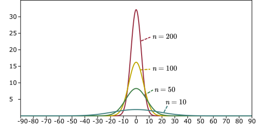
float normalization = (phongShininess + 2.0) * RECIPROCAL_2PI;
color += pow(specDot, phongShininess) * normalization * phongSpecularCol;
return color;
}
$\mathbf{l}$ $\mathbf{v}$ $k_d$ $k_s$ $n_s$

vec3 blinnPhongBRDF(vec3 lightDir, vec3 viewDir, vec3 normal,
            vec3 phongDiffuseCol, vec3 phongSpecularCol, float phongShininess) {
  vec3 color = phongDiffuseCol;
  vec3 halfDir = normalize(viewDir + lightDir);
  float specDot = max(dot(halfDir, normal), 0.0);
  color += pow(specDot, phongShininess) * phongSpecularCol;
  return color;
}
| Material | Index of Refraction | $\mathrm{F}_0$ |
|---|---|---|
| Vacuum | 1.0 | 0% |
| Air | 1.000292 | ≈ 0% |
| Water | 1.333 | 2% |
| Glass | 1.5 | 4% |
| Plastic | 1.5 to 1.58 | 4% to 5% |
| Diamond | 2.42 | 17.24% |
| Metals | $\mathrm{F}_0$ (Linear, Float) | $\mathrm{F}_0$ (sRGB, 8-bit) | Color |
|---|---|---|---|
| Titanium | (0.542, 0.497, 0.449) | (194, 187, 179) | |
| Chrome | (0.549, 0.556, 0.554) | (196, 197, 196) | |
| Iron | (0.562, 0.565, 0.578) | (198, 198, 200) | |
| Nickel | (0.660, 0.609, 0.526) | (212, 205, 192) | |
| Platinum | (0.673, 0.637, 0.585) | (214, 209, 201) | |
| Copper | (0.955, 0.638, 0.538) | (250, 209, 194) | |
| Palladium | (0.733, 0.697, 0.652) | (222, 217, 211) | |
| Zinc | (0.664, 0.824, 0.850) | (213, 234, 237) | |
| Gold | (1.022, 0.782, 0.344) | (255, 229, 158) | |
| Aluminum | (0.913, 0.922, 0.924) | (245, 246, 246) | |
| Silver | (0.972, 0.960, 0.915) | (252, 250, 245) |
#define RECIPROCAL_PI 0.3183098861837907
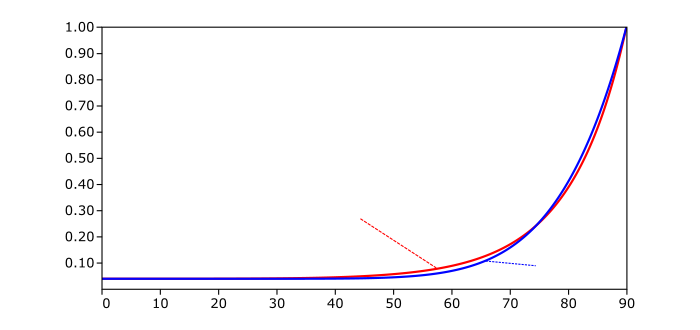
vec3 fresnelSchlick(float cosTheta, vec3 F0) {
return F0 + (1.0 - F0) * pow(1.0 - cosTheta, 5.0);
}
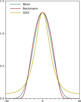
float D_GGX(float NoH, float roughness) {
float alpha = roughness * roughness;
float alpha2 = alpha * alpha;
float NoH2 = NoH * NoH;
float b = (NoH2 * (alpha2 - 1.0) + 1.0);
return alpha2 * RECIPROCAL_PI / (b * b);
}
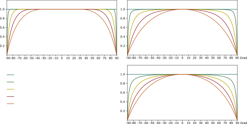
float G1_GGX_Schlick(float NoV, float roughness) {
float alpha = roughness * roughness;
float k = alpha / 2.0;
return max(NoV, 0.001) / (NoV * (1.0 - k) + k);
}
float G_Smith(float NoV, float NoL, float roughness) {
return G1_GGX_Schlick(NoL, roughness) * G1_GGX_Schlick(NoV, roughness);
}
float fresnelSchlick90(float cosTheta, float F0, float F90) {
return F0 + (F90 - F0) * pow(1.0 - cosTheta, 5.0);
}
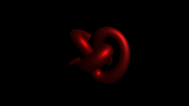
vec3 microfacetBRDF(in vec3 L, in vec3 V, in vec3 N,
in float metallic, in float roughness, in vec3 baseColor, in float reflectance) {
vec3 H = normalize(V + L);
float NoV = clamp(dot(N, V), 0.0, 1.0);
float NoL = clamp(dot(N, L), 0.0, 1.0);
float NoH = clamp(dot(N, H), 0.0, 1.0);
float VoH = clamp(dot(V, H), 0.0, 1.0);
vec3 f0 = vec3(0.16 * (reflectance * reflectance));
f0 = mix(f0, baseColor, metallic);
vec3 F = fresnelSchlick(VoH, f0);
float D = D_GGX(NoH, roughness);
float G = G_Smith(NoV, NoL, roughness);
vec3 spec = (F * D * G) / (4.0 * max(NoV, 0.001) * max(NoL, 0.001));
vec3 rhoD = baseColor;
// optionally
rhoD *= vec3(1.0) - F;
rhoD *= (1.0 - metallic);
vec3 diff = rhoD * RECIPROCAL_PI;
return diff + spec;
}

Please notify me by e-mail if you have questions, suggestions for improvement, or found typos: Contact