Graphics Programming
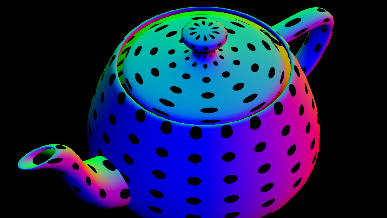
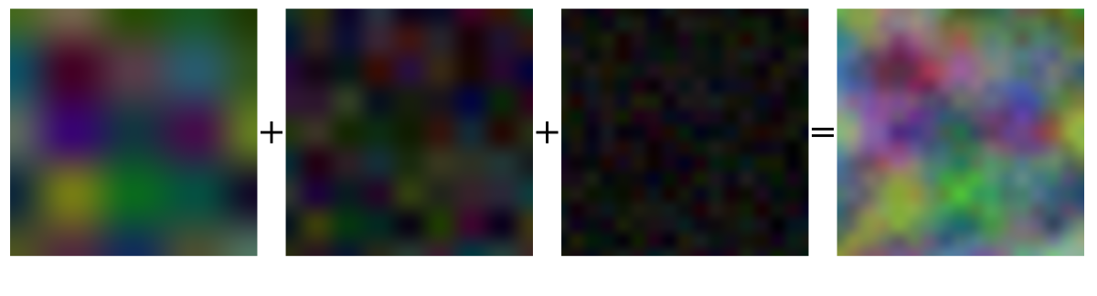
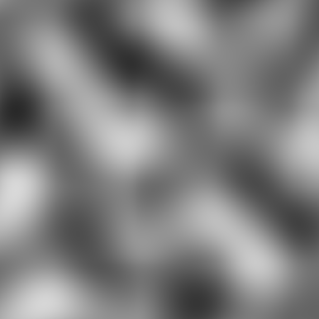
Procedural Textures and Noise
Thorsten Thormählen
January 26, 2026
Part 11, Chapter 1
Thorsten Thormählen
January 26, 2026
Part 11, Chapter 1
This is the print version of the slides.
Advance slides with the → key or
by clicking on the right border of the slide
Slides can also be advanced by clicking on the left or right border of the slide.
| Type | Font | Examples |
|---|---|---|
| Variables (scalars) | italics | $a, b, x, y$ |
| Functions | upright | $\mathrm{f}, \mathrm{g}(x), \mathrm{max}(x)$ |
| Vectors | bold, elements row-wise | $\mathbf{a}, \mathbf{b}= \begin{pmatrix}x\\y\end{pmatrix} = (x, y)^\top,$ $\mathbf{B}=(x, y, z)^\top$ |
| Matrices | Typewriter | $\mathtt{A}, \mathtt{B}= \begin{bmatrix}a & b\\c & d\end{bmatrix}$ |
| Sets | calligraphic | $\mathcal{A}, B=\{a, b\}, b \in \mathcal{B}$ |
| Number systems, Coordinate spaces | double-struck | $\mathbb{N}, \mathbb{Z}, \mathbb{R}^2, \mathbb{R}^3$ |
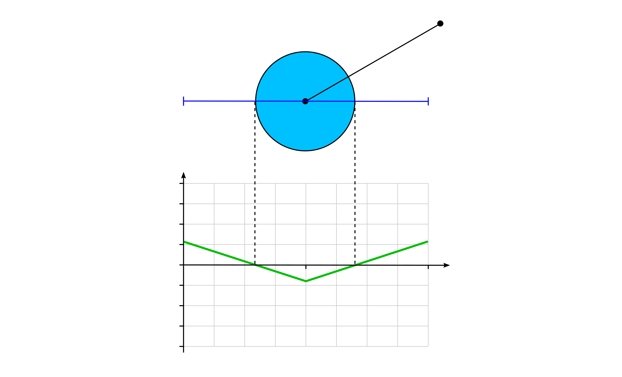
float fill(float sdf) {
    return step(0.0, -sdf);
}float stroke(float sdf, float strokeWidth) {
return fill(abs(sdf) - strokeWidth);
}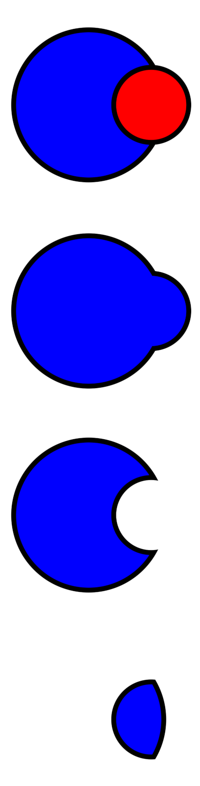
float unionSDF(float sdf0, float sdf1) {
  return min(sdf0, sdf1);
}float differenceSDF(float sdf0, float sdf1) {
return max(sdf0, -sdf1);
}float intersectionSDF(float sdf0, float sdf1) {
return max(sdf0, sdf1);
}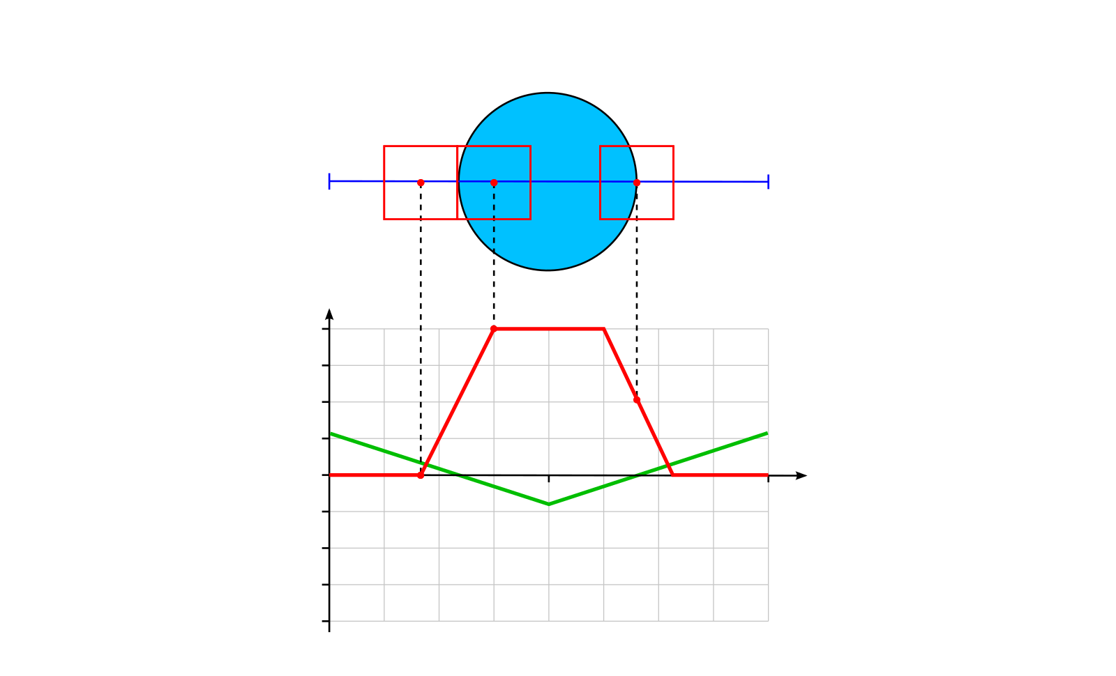
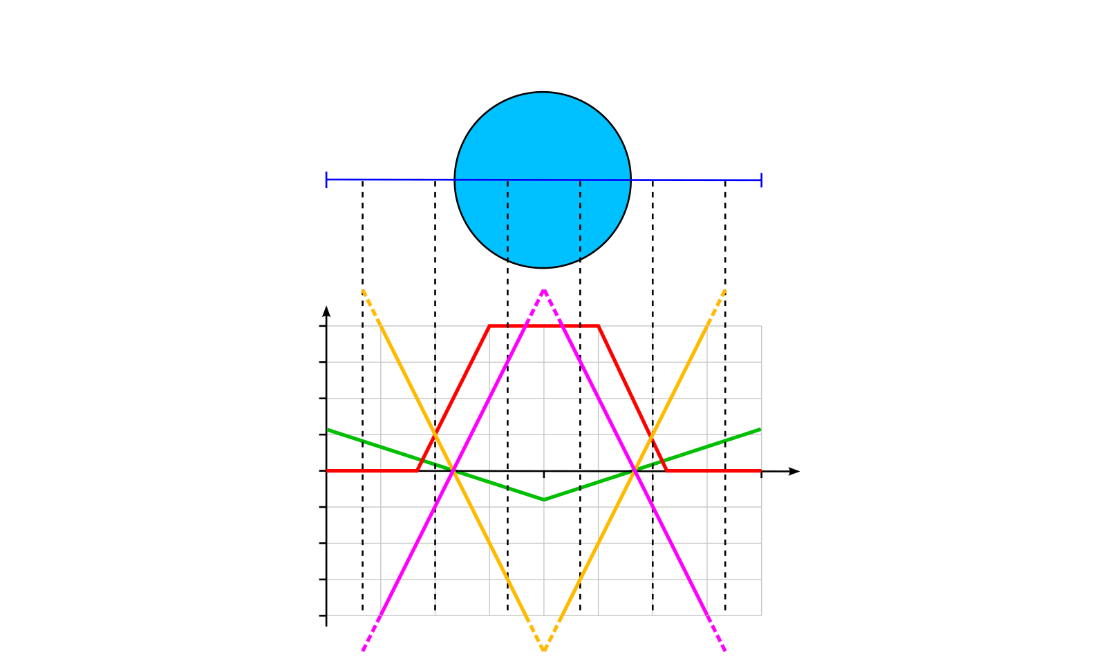
float fill(float sdf) {
  return clamp(0.5 - sdf / fwidth(sdf), 0.0, 1.0);
}float stroke(float sdf, float strokeWidth) {
return fill(abs(sdf) - strokeWidth);
}
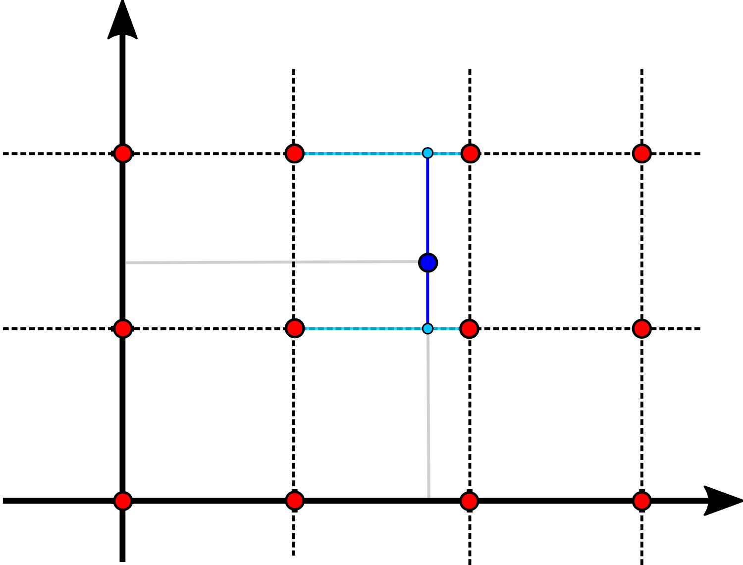
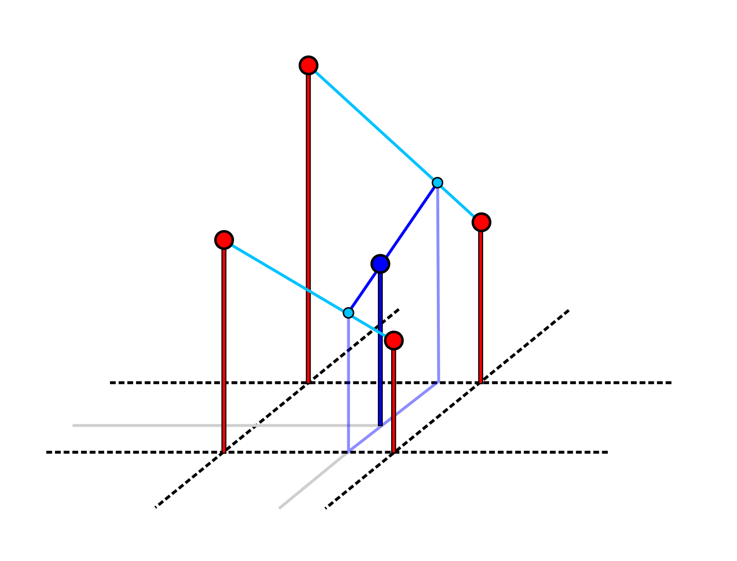
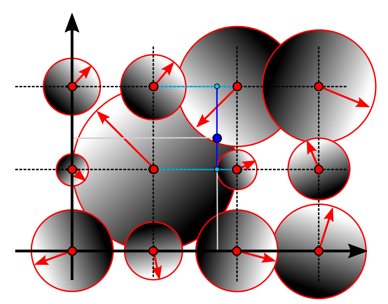
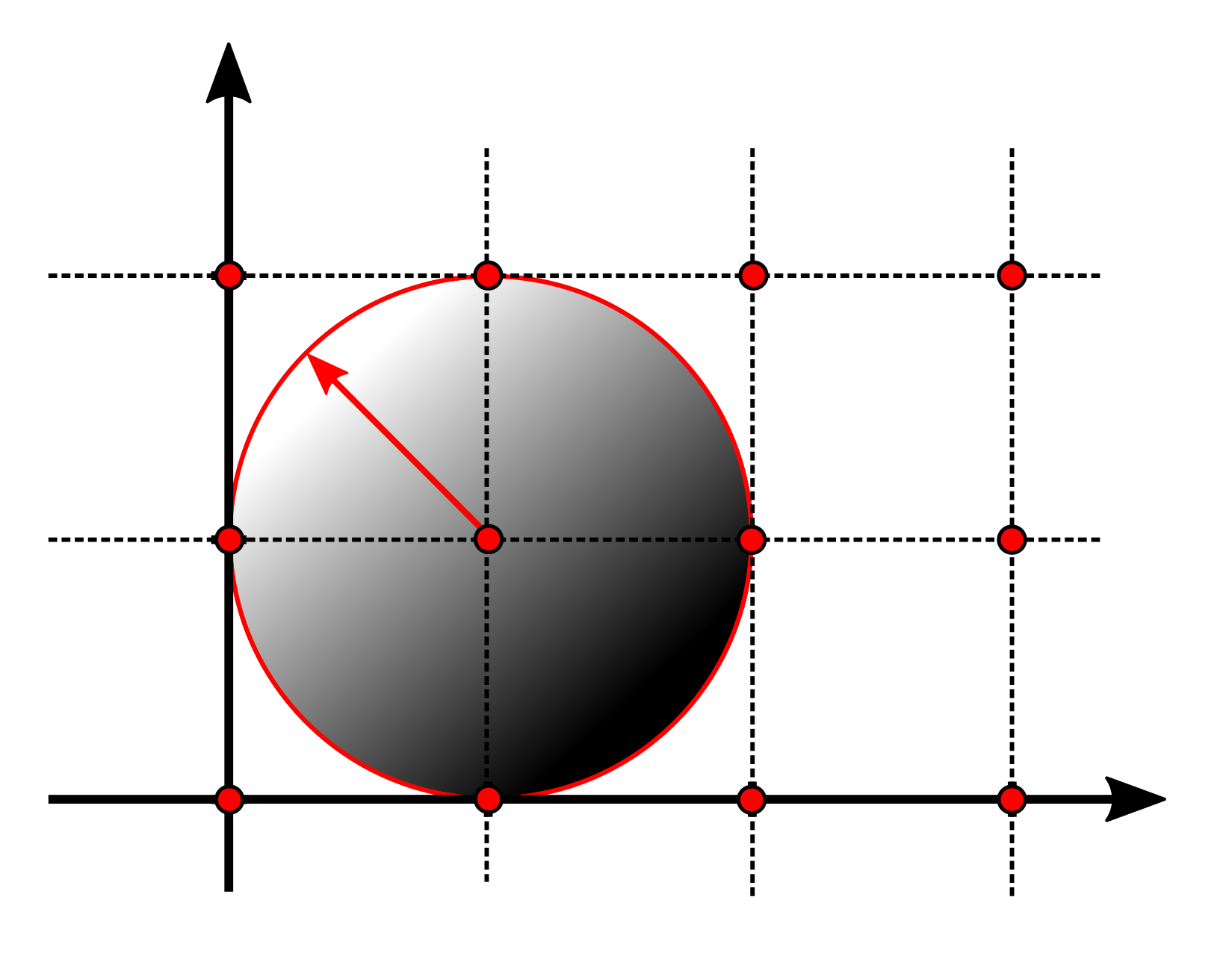
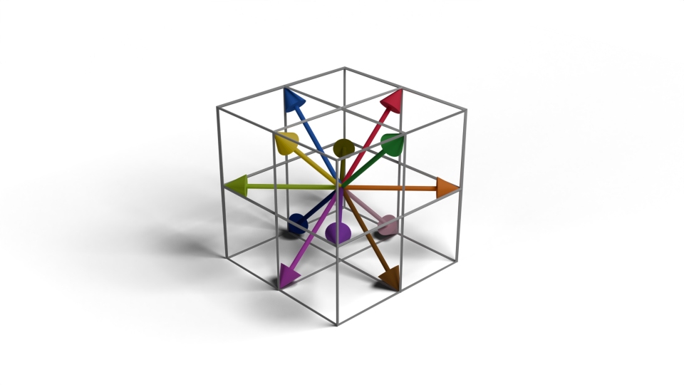
vec3 random_pcg3d(uvec3 v) {
  v = v * 1664525u + 1013904223u;
  v.x += v.y*v.z; v.y += v.z*v.x; v.z += v.x*v.y;
  v ^= v >> 16u;
  v.x += v.y*v.z; v.y += v.z*v.x; v.z += v.x*v.y;
  return vec3(v) * (1.0/float(0xffffffffu));
}
uvec3 are "shuffled" by multiplication with large prime numbers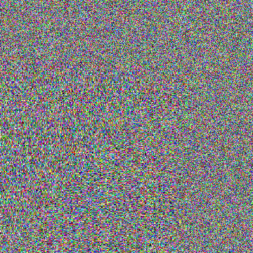
$\mathrm{f}(x) = 3 x^2 - 2 x^3 = x^2 (3 - 2 x)$

smoothstep(0.0, 1.0, x) 
$\mathrm{f}(x) = 6 x^5 - 15 x^4 + 10 x^3 = x^3\,(x\,(6\,x - 15)+10)$

smoothstep smootherstep 
Please notify me by e-mail if you have questions, suggestions for improvement, or found typos: Contact