Control Keys

move to next slide (also Enter or Spacebar).
move to previous slide.
 d  enable/disable drawing on slides
 p  toggles between print and presentation view
CTRL  +  zoom in
CTRL  -  zoom out
CTRL  0  reset zoom

Slides can also be advanced by clicking on the left or right border of the slide.

Notation

Type Font Examples
Variables (scalars) italics $a, b, x, y$
Functions upright $\mathrm{f}, \mathrm{g}(x), \mathrm{max}(x)$
Vectors bold, elements row-wise $\mathbf{a}, \mathbf{b}= \begin{pmatrix}x\\y\end{pmatrix} = (x, y)^\top,$ $\mathbf{B}=(x, y, z)^\top$
Matrices Typewriter $\mathtt{A}, \mathtt{B}= \begin{bmatrix}a & b\\c & d\end{bmatrix}$
Sets calligraphic $\mathcal{A}, B=\{a, b\}, b \in \mathcal{B}$
Number systems, Coordinate spaces double-struck $\mathbb{N}, \mathbb{Z}, \mathbb{R}^2, \mathbb{R}^3$

Introduction: Object Transformations

  • In computer graphics objects are often used multiple times. The same geometry is "transformed" and appears
    • at various positions, e.g. repetitive windows in a building
    • in various sizes, e.g. a S, L or XL pop corn container
    • in different orientations, e.g. the orientation of a person's hand
  • Also, the position, orientation, and size of an object can change over time, e.g., the limbs of a running person

Example

  • The scooter changes its position over time
  • The wheels change their orientation
  • A wheel consists of several spokes with the same geometry. Thus, this geometry must be stored only once. The other spokes can be transformed references.
Source: : 3D model:Dosch Design; Renderer: Mental Ray / 3ds Max 2010;

2D Transformations

2D Translation

translation
$\mathbf{p}$
$\tilde{\mathbf{p}}$
$\mathbf{t}$
object
translated object
$x$
$y$
  • A change in position of an object can be achieved by a translation
  • Given: A vertex point $\mathbf{p}=(x,y)^\top$ of an object
  • When moving the object around $t_x$ in x-direction and $t_y$ in y-direction, the new coordinates $\tilde{\mathbf{p}}$ of the vertex are given by:

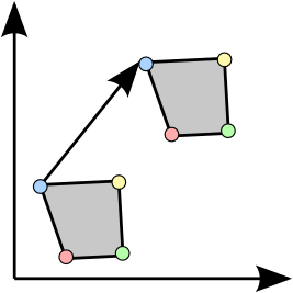
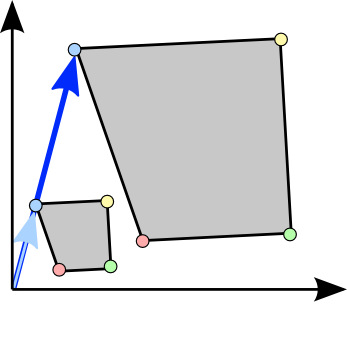
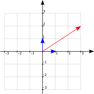
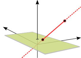
$\tilde{\mathbf{p}}= \begin{pmatrix} \tilde{x}\\ \tilde{y}\end{pmatrix} = \begin{pmatrix} x + t_x\\ y + t_y \end{pmatrix} = \mathbf{p} + \begin{pmatrix} t_x\\ t_y \end{pmatrix} = \mathbf{p} + \mathbf{t}$
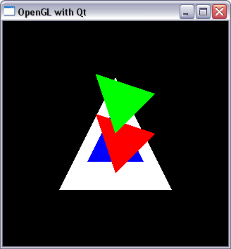
2D Scaling

scale
$\mathbf{p}$
$\tilde{\mathbf{p}}$
object
scaled object
$x$
$y$
  • A change in size of an object can be achieved by scaling
  • A magnification of the object by a factor of $s$ is given by:
    $\tilde{\mathbf{p}}= \begin{pmatrix} s \, x \\ s \, y\end{pmatrix} = s \, \mathbf{p}$
  • or in the case of non-uniform scaling in x- and y-direction:
    $\tilde{\mathbf{p}}= \begin{pmatrix} s_x \, x \\ s_y \, y\end{pmatrix} = \begin{bmatrix} s_x & 0 \\ 0 & s_y\end{bmatrix} \mathbf{p}$

2D Rotation

  • When rotating a coordinate system by the angle $\alpha$, the rotated coordinate axes are given by:
    $\tilde{\mathbf{b}}_x = \begin{pmatrix} \cos \alpha \\ \sin \alpha \end{pmatrix}$ and  $\tilde{\mathbf{b}}_y = \begin{pmatrix} -\sin \alpha\\ \cos \alpha \end{pmatrix}$
rotation
$\tilde{\mathbf{b}}_x$
$\tilde{\mathbf{b}}_y$
object
rotated object
$\alpha$
$x$
$y$
1
$\cos \alpha$
$$\sin \alpha$$

2D Rotation

  • To rotate an object, the given vertex coordinates $\mathbf{p}=(x,y)^\top$ can be displayed in the rotated coordinate system. Then the rotated point $\tilde{\mathbf{p}}$ can be expressed in the original coordinate system by:
    $ \begin{aligned} \tilde{\mathbf{p}} &= \tilde{\mathbf{b}}_x \, x + \tilde{\mathbf{b}}_y\, y = \begin{pmatrix} \cos \alpha \\ \sin \alpha \end{pmatrix} x + \begin{pmatrix} -\sin \alpha\\ \cos \alpha \end{pmatrix} y \\ &= \underbrace{\begin{bmatrix}\tilde{\mathbf{b}}_x & \tilde{\mathbf{b}}_y \end{bmatrix}}_{\mathtt{R}} \begin{pmatrix}x \\ y \end{pmatrix} = \underbrace{\begin{bmatrix}\cos \alpha & -\sin \alpha\\ \sin \alpha & \cos \alpha \end{bmatrix}}_{\mathtt{R}} \begin{pmatrix}x \\ y \end{pmatrix}\\ &= \mathtt{R} \, \mathbf{p} \end{aligned} $

Combination of Translation, Scaling, and Rotation

  • If an object should be first scaled, then rotated, and lastly translated, the following applies:
    $\tilde{\mathbf{p}} = \mathtt{R} \, s \, \mathbf{p} + \mathbf{t}$
  • Does this give the same result as:
    $\tilde{\mathbf{p}} = \mathtt{R} \, s \, (\mathbf{p} + \mathbf{t})$ ?
  • No, the order is important!
    compare_order

2D Transformations in OpenGL

opengl_triangletranform

2D Transformations in OpenGL

class Renderer {
private:
    void drawTriangle() {
        glBegin(GL_TRIANGLES);
        glVertex3f(-0.5f, -0.5f, 0.0f);
        glVertex3f( 0.5f, -0.5f, 0.0f);
        glVertex3f( 0.0f,  0.5f, 0.0f);
        glEnd();
    }

public:
    void init() {}
    void resize(int w, int h) {
        glViewport(0, 0, w, h);
    }
    void display() {
        glClearColor(0.0f, 0.0f, 0.0f, 0.0f);
        glClear(GL_COLOR_BUFFER_BIT);
        glOrtho(-1.0f, 1.0f, -1.0f, 1.0f, -1.0f, 1.0f);
        glLoadIdentity();
        glColor3f(1.0f, 1.0f, 1.0f);
        drawTriangle();

        glColor3f(0.0f, 0.0f, 1.0f);
        glScalef(0.5, 0.5, 0.0); // resize to 50%
        drawTriangle();

        glColor3f(1.0f, 0.0f, 0.0f);
        glRotatef(45.0, 0.0, 0.0, 1.0); //rotate 45 degrees
        drawTriangle();

        glColor3f(0.0f, 1.0f, 0.0f);
        glTranslatef(0.5, 0.5, 0.0); // translate
        drawTriangle();
    }
    void dispose() {}
};

Desire for Unification

  • Currently, depending on the type of transformation (rotation, scaling, or translation) different operations are performed (matrix multiplication, vector scaling, and vector addition)
  • It will turn out that transformations can be generally realized by matrix multiplications, i.e. all three operation can be expressed by $\tilde{\mathbf{p}} = \mathtt{T} \, \mathbf{p}$
  • In order to achieve this, some mathematical fundamentals will be taught in the following. Particularly important in this context are "linear mappings" and "homogeneous coordinates"

Linear Mappings

Linear Combination

  • If multiple vectors $\mathbf{v}_i$ of a vector space are multiplied by scalars and are summed up, the result is a so-called linear combination:
    $\mathbf{v} = \sum\limits_{i=1}^n a_i \mathbf{v}_i$
  • All possible linear combinations form the span of the vectors:
    $ \ll \mathbf{v}_i \gg \,\, = \left\{ \sum\limits_{i=1}^n a_i \mathbf{v}_i \, | \,a_i \in \mathbb{R} \right\}$
  • Vectors are linearly independent if no vector can be represented as a linear combination of the others
  • The maximum number of $n$ linearly independent vectors forms a basis of the vector space
  • The vectors of a basis are called base vectors and are typically denoted by $\mathbf{b}$ in the lecture
  • The number $n$ of base vectors is called the dimension of the vector space

Linear Combination

  • An example for a basis of the $\mathbb{R}^2$ are, for example, the unit vectors
    $\mathbf{b}_1=\mathbf{e}_x = \begin{pmatrix}1 \\ 0 \end{pmatrix}$ und $\mathbf{b}_2 = \mathbf{e}_y = \begin{pmatrix}0 \\ 1 \end{pmatrix}$,
    because by their linear combination every possible vector $\mathbf{v}=(x, y)^\top$ of the vector space can be generated:
    $\mathbf{v} = \begin{pmatrix}x \\ y \end{pmatrix} = x \, \mathbf{e}_x + y \, \mathbf{e}_y = x \begin{pmatrix}1 \\ 0 \end{pmatrix} + y \begin{pmatrix}0 \\ 1 \end{pmatrix}$
  • Another possible basis of the $\mathbb{R}^2$ are the vectors
    $\mathbf{b}_1=\begin{pmatrix}2 \\ 1 \end{pmatrix}$ und $\mathbf{b}_2 = \begin{pmatrix}0 \\ -1 \end{pmatrix}$
    because also by their linear combination every possible vector can be generated

Linear Combination

basetransform0
$x$
$y$
$\mathbf{e}_x$
$\mathbf{e}_y$
  • A 2-vector, as here for example $(3, 2)^\top$, is usually interpreted as a point in the Cartesian coordinate system, i.e., it is the linear combination
    $3 \, \mathbf{e}_x + 2 \, \mathbf{e}_y $
  • However, the 2-vector $(3, 2)^\top$ could also mean something completely different, for example:
    $3 \, \begin{pmatrix}2 \\ 1 \end{pmatrix} + 2 \, \begin{pmatrix}0 \\ -1 \end{pmatrix} $
  • This means that when a vector is given, it must always be said in which vector space it is to be interpreted

Linear Mapping

  • Given a mapping function $\mathrm{f}: \mathcal{V}\rightarrow \tilde{\mathcal{V}}$ that maps a vector space  $\mathcal{V}$ into another vector space $\tilde{\mathcal{V}}$ and a joint field $\mathcal{K}$.
  • This mapping is called a linear mapping if for all vectors $\mathbf{v}_1, \mathbf{v}_2 \in \mathcal{V}$ and scalar $a \in \mathcal{K}$ it holds:
    $\mathrm{f}(\mathbf{v}_1 + \mathbf{v}_2) = \mathrm{f}(\mathbf{v}_1) + \mathrm{f}(\mathbf{v}_2)$ and
    $\mathrm{f}(a \mathbf{v}_1) = a \, \mathrm{f}(\mathbf{v}_1)$
  • For linear combinations under a linear mapping it follows that:
    $\mathrm{f}\left(\sum\limits_{i=1}^n a_i \mathbf{v}_i\right) = \sum\limits_{i=1}^n a_i \mathrm{f}(\mathbf{v}_i)$

Linear Mapping

  • A linear mapping $\mathrm{f}$ is uniquely defined by the mapping of the base vectors $\mathrm{f}(\mathbf{b}_i)$. It holds that:
    $\mathbf{v} = \sum\limits_{i=1}^n a_i \mathbf{b}_i \rightarrow \mathrm{f}(\mathbf{v}) = \sum\limits_{i=1}^n a_i \mathrm{f}(\mathbf{b}_i) \quad \forall \mathbf{v} \in \mathcal{V}$

Linear Mapping

  • A linear mapping $\mathrm{f}$ can be expressed as a matrix-vector multiplication. Example:
    $\tilde{\mathbf{v}} = \mathrm{f}(\mathbf{v}) = \begin{pmatrix}\tilde{v}_x \\ \tilde{v}_y \end{pmatrix} = \underbrace{\begin{bmatrix}m_{11} & m_{12}\\ m_{21} & m_{22} \end{bmatrix}}_{\mathtt{M}} \begin{pmatrix}v_x \\ v_y \end{pmatrix} = \mathtt{M} \, \mathbf{v}$
  • In general, it is a $M \times N$ matrix: $\begin{pmatrix}\tilde{v}_1 \\ \vdots \\\tilde{v}_M \end{pmatrix} = \begin{pmatrix} m_{1,1} & m_{1,2} & \cdots & m_{1,N} \\ m_{2,1} & m_{2,2} & \cdots & m_{2,N} \\ \vdots & \vdots & \ddots & \vdots \\ m_{M,1} & m_{M,2} & \cdots & m_{M,N} \end{pmatrix} \begin{pmatrix}v_1 \\ \vdots \\ v_N \end{pmatrix}$

Linear Mapping

  • In the columns of the matrix $\mathtt{M}$ the mappings of the base vectors in the current reference coordinate system can be read off.
    $\mathtt{M} = \begin{bmatrix}m_{11} & m_{12}\\ m_{21} & m_{22} \end{bmatrix} = \begin{bmatrix}\tilde{\mathbf{b}}_x & \tilde{\mathbf{b}}_y \end{bmatrix}$
  • Assuming the reference coordinate system is spanned by:
    $\mathbf{e}_x = \begin{pmatrix}1 \\ 0 \end{pmatrix}$ und $\mathbf{e}_y = \begin{pmatrix}0 \\ 1 \end{pmatrix}$
  • Then we have:
    $\tilde{\mathbf{b}}_x = \mathrm{f}(\mathbf{e}_x) = \begin{bmatrix}m_{11} & m_{12}\\ m_{21} & m_{22} \end{bmatrix} \begin{pmatrix}1 \\ 0 \end{pmatrix} = \begin{pmatrix}m_{11} \\ m_{21} \end{pmatrix}$ and
    $\tilde{\mathbf{b}}_y = \mathrm{f}(\mathbf{e}_y) = \begin{bmatrix}m_{11} & m_{12}\\ m_{21} & m_{22} \end{bmatrix} \begin{pmatrix}0 \\ 1 \end{pmatrix} = \begin{pmatrix}m_{12} \\ m_{22} \end{pmatrix}$
  • Therefore, when designing a particular transformation, the sole consideration must be how to map the base vectors (see, e.g., the derivation of the rotation matrix at the beginning of this chapter)

Example 1

basetransform1
$x$
$y$
$\mathbf{e}_x$
$\mathbf{e}_y$
$\tilde{\mathbf{b}}_x$
$\tilde{\mathbf{b}}_y$
$\mathbf{p}$
  • Base vectors of the reference basis:
    $\mathbf{e}_x = \begin{pmatrix}1 \\ 0 \end{pmatrix}$, $\mathbf{e}_y = \begin{pmatrix}0 \\ 1 \end{pmatrix}$
  • Base vectors of the new basis:
    $\tilde{\mathbf{b}}_x = \begin{pmatrix}2 \\ 2 \end{pmatrix}$, $\tilde{\mathbf{b}}_y = \begin{pmatrix}-2 \\ 2 \end{pmatrix}$
  • What is the corresponding transformation matrix?
  • The transformation matrix is given by the new base vectors in the reference coordinate system:
    $\mathtt{T}=\begin{bmatrix}\tilde{\mathbf{b}}_x & \tilde{\mathbf{b}}_y \end{bmatrix} = \begin{bmatrix}2 & -2\\ 2 & 2 \end{bmatrix}$
  • What are the coordinates of the transformed point?
  • $\mathbf{p}=\begin{pmatrix}2 \\ 1 \end{pmatrix} \rightarrow \tilde{\mathbf{p}} = \mathtt{T}\, \mathbf{p} = \begin{bmatrix}2 & -2\\ 2 & 2 \end{bmatrix} \begin{pmatrix}2 \\ 1 \end{pmatrix} = \begin{pmatrix}2 \\ 6 \end{pmatrix}$

Example 2

basetransform2
$x$
$y$
$\mathbf{b}_x$
$\mathbf{b}_y$
$\tilde{\mathbf{b}}_x$
$\tilde{\mathbf{b}}_y$
$\mathbf{p}$
  • Base vectors of the reference basis:
    $\mathbf{b}_x = (2, -1)^\top$, $\mathbf{b}_y = (-1, 2)^\top$
  • Base vectors of the new basis in the global coordinate system:
    $\tilde{\mathbf{b}}_x = (3, 0)^\top$, $\tilde{\mathbf{b}}_y = (1, -2)^\top$
  • What are the new base vectors expressed by the base vectors of the reference basis?
  • $\tilde{\mathbf{b}}_x = 2 \mathbf{b}_x + \mathbf{b}_y$, $\tilde{\mathbf{b}}_y = 0 \mathbf{b}_x + (-1) \mathbf{b}_y$
  • In the reference coordinate system we have:
    $\mathtt{T}= \begin{bmatrix} 2& 0\\ 1 & -1 \end{bmatrix}$
    $\mathbf{p} = \begin{pmatrix}-1 \\ 0 \end{pmatrix} \rightarrow \tilde{\mathbf{p}} = \mathtt{T}\, \mathbf{p} = \begin{bmatrix}2 & 0\\ 1 & -1 \end{bmatrix} \begin{pmatrix}-1 \\ 0 \end{pmatrix} = \begin{pmatrix}-2 \\ -1 \end{pmatrix}$
  • In the global coordinate system this results in:
    $\tilde{\mathbf{p}} = -2 \mathbf{b}_x + (-1) \mathbf{b}_y = (-3, 0)^\top$

Homogeneous Coordinates

Homogeneous Coordinates

  • As the example has shown, scaling and rotation can be represented in $\mathbb{R}^2$ by a linear mapping using a $2 \times 2$ matrix $\mathtt{M}$. Thus, a rotation and scaling by matrix multiplication is already achieved:
    $\tilde{\mathbf{p}} = \mathtt{M} \,\mathbf{p}$
  • If a point should be additionally translated, the translation vector $\mathbf{t}$ must be added
    $\tilde{\mathbf{p}} = \mathtt{M} \,\mathbf{p} + \mathbf{t}$
  • The use of homogeneous coordinates allows to further unify the formulation and to implement the translation also as a linear mapping (matrix multiplication)

Homogeneous Coordinates

  • Trick: A point $\mathbf{p}$ is no longer represented as a 2-vector $\mathbf{p}=(x,y)^\top \in \mathbb{R}^2$ but receives an additional component
    $\underline{\mathbf{p}}=\begin{pmatrix} x \\ y \\ 1 \end{pmatrix} \in \mathbb{H}^2$
  • This is a representation of the point in homogeneous coordinates
  • It allows a transformed point $\underline{\tilde{\mathbf{p}}}$ to be expressed as:
    $\underline{\tilde{\mathbf{p}}} = \begin{pmatrix} \tilde{x} \\ \tilde{y} \\ 1 \end{pmatrix} = \begin{bmatrix}m_{11} & m_{12} & t_x\\ m_{21} & m_{22} & t_y \\ 0 & 0 & 1\end{bmatrix} \begin{pmatrix} x \\ y \\ 1 \end{pmatrix} $
    $\underline{\tilde{\mathbf{p}}} = \underbrace{\begin{bmatrix}\mathtt{M}& \mathbf{t} \\ \mathbf{0} & 1\end{bmatrix}}_{ \mathtt{T}} \underline{\mathbf{p}}$
    $\underline{\tilde{\mathbf{p}}} = \mathtt{T} \underline{\mathbf{p}}$
  • Thus, the consistent application of transformations (rotation, scaling, and translation) as matrix-vector multiplication is achieved

Homogeneous Coordinates

  • If the last row of the matrix $\mathtt{T}$ is not of the special form $(0, 0, 1)$, the third coordinate of $\underline{\tilde{\mathbf{p}}}$ is not necessarily equal to 1
    $\underline{\tilde{\mathbf{p}}} = \begin{pmatrix} u \\ v \\ w \end{pmatrix} = \begin{bmatrix}t_{11} & t_{12} & t_{13}\\ t_{21} & t_{22} & t_{23} \\ t_{31} & t_{32} & t_{33}\end{bmatrix} \begin{pmatrix} x \\ y \\ 1 \end{pmatrix} $
  • In this case, the Cartesian coordinates $(x, y)^\top$ can not be read off directly from the homogeneous coordinates
  • Instead the following conversion of a homogeneous point into Cartesian coordinates is applied:
    $\underline{\mathbf{p}}=\begin{pmatrix} u \\ v \\ w \end{pmatrix} \in \mathbb{H}^2 \rightarrow \mathbf{p} = \begin{pmatrix} x \\ y \\ \end{pmatrix} = \begin{pmatrix} \frac{u}{w} \\ \frac{v}{w} \\ \end{pmatrix} \in \mathbb{R}^2$
  • If the homogeneous point is scaled by a factor of $\lambda$, this has no effect on the Cartesian coordinates:
    $\lambda \underline{\mathbf{p}}=\begin{pmatrix} \lambda u \\ \lambda v \\ \lambda w \end{pmatrix} \in \mathbb{H}^2 \rightarrow \mathbf{p} = \begin{pmatrix} x \\ y \\ \end{pmatrix} = \begin{pmatrix} \frac{\lambda u}{\lambda w} \\ \frac{\lambda v}{\lambda w} \\ \end{pmatrix} = \begin{pmatrix} \frac{u}{w} \\ \frac{v}{w} \\ \end{pmatrix} \in \mathbb{R}^2$

Homogeneous Coordinates

homogenous_projection
plane $z=1$
$x$
$y$
$z$
$\mathbb{R}^3$ or $\mathbb{H}^2$
$\lambda \underline{\mathbf{p}}$
$\mathbf{p}$
  • That is, when scaled with $\lambda=\frac{1}{w}$ the first two coordinates of a homogeneous point directly correspond to the Cartesian coordinates
    $\lambda \underline{\mathbf{p}}=\begin{pmatrix} \lambda u \\ \lambda v \\ \lambda w \end{pmatrix} = \begin{pmatrix} x \\ y\\ 1 \end{pmatrix}$, wenn $\lambda=\frac{1}{w}$
  • When interpreting $\underline{\mathbf{p}}$ as an element of $\mathbb{R}^3$ the scaling with $\lambda=\frac{1}{w}$ can be geometrically interpreted as a projection of a point onto the plane $z=1$
  • Due to this property, the homogeneous coordinates are the fundamental entities of the so-called projective geometry, which will later be especially interesting for the geometric description of cameras
  • All points along the line from the origin to point $\underline{\mathbf{p}}$ are mapped to the same point on the plane $z=1$
  • This means that each element of $\mathbb{R}^2$ corresponds to a straight line in $\mathbb{H}^2$

Classification of Transformations

tranformation_compare
translational
isometric
similar
affine
projective
  • Translation; Translation and rotation (Isometries)
    $\mathtt{T} = \begin{bmatrix}1 & 0& t_x\\ 0 & 1 & t_y \\ 0 & 0 &1\end{bmatrix}$; $\mathtt{T} = \begin{bmatrix} \cos \alpha & - \sin \alpha & t_x\\ \sin \alpha & \cos \alpha & t_y \\ 0 & 0 &1\end{bmatrix} $
  • Translation, rotation, and scaling (Similarity)
    $\mathtt{T} = \begin{bmatrix} s \cos \alpha & -s \sin \alpha & t_x\\ s \sin \alpha & s \cos \alpha & t_y \\ 0 & 0 &1\end{bmatrix} $
  • Affine transformation
    $\mathtt{T} = \begin{bmatrix} t_{11} & t_{12} & t_{13}\\ t_{21} & t_{22} & t_{23} \\ 0 & 0 &1\end{bmatrix} $
  • Projektive transformation
    $\mathtt{T} = \begin{bmatrix} t_{11} & t_{12} & t_{13}\\ t_{21} & t_{22} & t_{23} \\ t_{31} & t_{32} & t_{33}\end{bmatrix} $

Are there any questions?

questions

Please notify me by e-mail if you have questions, suggestions for improvement, or found typos: Contact

More lecture slides

Slides in German (Folien auf Deutsch)