Bildsynthese
Intersection Shader
Thorsten Thormählen
05. Mai 2026
Teil 2, Kapitel 2
Thorsten Thormählen
05. Mai 2026
Teil 2, Kapitel 2
Dies ist die Druck-Ansicht.
Weiterschalten der Folien durch die → Taste oder
durch das Klicken auf den rechten Folienrand.
Das Weiterschalten der Folien kann ebenfalls durch das Klicken auf den rechten bzw. linken Folienrand erfolgen.
| Typ | Schriftart | Beispiele |
|---|---|---|
| Variablen (Skalare) | kursiv | $a, b, x, y$ |
| Funktionen | aufrecht | $\mathrm{f}, \mathrm{g}(x), \mathrm{max}(x)$ |
| Vektoren | fett, Elemente zeilenweise | $\mathbf{a}, \mathbf{b}= \begin{pmatrix}x\\y\end{pmatrix} = (x, y)^\top,$ $\mathbf{B}=(x, y, z)^\top$ |
| Matrizen | Schreibmaschine | $\mathtt{A}, \mathtt{B}= \begin{bmatrix}a &b\\c &d\end{bmatrix}$ |
| Mengen | kalligrafisch | $\mathcal{A}, B=\{a, b\}, b \in \mathcal{B}$ |
| Zahlenbereiche, Koordinatenräume | doppelt gestrichen | $\mathbb{N}, \mathbb{Z}, \mathbb{R}^2, \mathbb{R}^3$ |

reportIntersectionEXT(...)hitAttributeEXT Variable schreiben, die vom benutzerdefinierten Typ ist
und im Closest-Hit oder Any-Hit Shader
ausgewertet werden kann
struct HitAttributeType {
vec3 normal;
vec2 texCoord;
}; // type of the "hit" variable
...
void main() { /**** INTERSECTION SHADER ****/
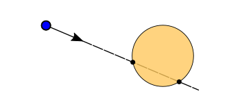
// ray-sphere intersection in world space
// get bounding box in object space
vec3 aabbMin;
vec3 aabbMax;
gsnGetIntersectionBox(gl_InstanceID, gl_PrimitiveID, aabbMin, aabbMax);
// transform to world space
vec3 minWorld = gl_ObjectToWorldEXT * vec4(aabbMin, 1.0);
vec3 maxWorld = gl_ObjectToWorldEXT * vec4(aabbMax, 1.0);
// center and radius of sphere in world space
vec3 center = (minWorld + maxWorld) / 2.0;
float radius = length((maxWorld - minWorld) / (sqrt(3.0) * 2.0));
vec3 b = gl_WorldRayOriginEXT - center;
vec3 r = normalize(gl_WorldRayDirectionEXT);
float p = 2.0 * dot(r, b);
float q = dot(b, b) - radius * radius;
// discriminant of the quadratic equation
float d =(p * p / 4.0) - q;
// if no solution, cancel computation
if(d < 0.0) return;
// two solutions for quadratic equation
float tin = -p / 2.0 - sqrt(d);
float tout = -p / 2.0 + sqrt(d);
// intersection at tin or tout?
float t = tout;
uint hitKind = 2u;
if(tin < tout && tin >= gl_RayTminEXT && tin <= gl_RayTmaxEXT) {
t = tin;
hitKind = 1u;
}
if(t >= gl_RayTminEXT && t <= gl_RayTmaxEXT) {
vec3 hitPoint = gl_WorldRayOriginEXT + t * gl_WorldRayDirectionEXT;
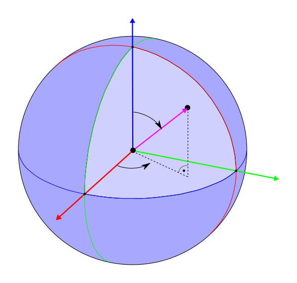
vec3 n = normalize(hitPoint - center);
vec3 localN = normalize(gl_WorldToObjectEXT * vec4(n, 0.0));
hit.normal = n;
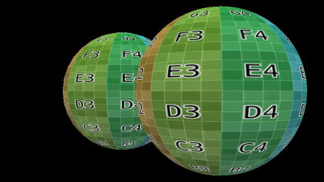
hit.texCoord.s = fract(atan(localN.y, localN.x) / (2.0 * PI));
hit.texCoord.t = acos(-localN.z) / (PI);
reportIntersectionEXT(t, hitKind);
}
}
gl_ObjectToWorldEXTgl_WorldToObjectEXTgl_InstanceID = 0gl_InstanceID = 1gl_InstanceID = 2reportIntersectionEXT(...)
den Wert für $t$ im Weltkoordinatensystem erwartet. Außerdem sind
gl_RayTminEXT und
gl_RayTmaxEXT ebenfalls im Weltkoordinatensystem definiert.
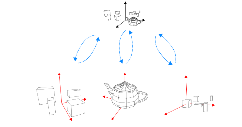
gl_ObjectToWorldEXT ist eine 3 x 4 Matrix, d.h. sie
enthält nur die obersten drei Zeilen von $\mathtt{T}$
gl_WorldToObjectEXT ist eine 3 x 4 Matrix, d.h. sie
enthält nur die obersten drei Zeilen von $\mathtt{T}^{-1}$
gl_ObjectRayOriginEXT
und $\tilde{\mathbf{r}}$ durch gl_ObjectRayDirectionEXT bereit gestelltgl_WorldRayOriginEXT $\,\mathbf{s}$ und gl_WorldRayDirectionEXT $\,\mathbf{r}$
gl_ObjectRayOriginEXT $\,\tilde{\mathbf{s}}$ und gl_ObjectRayDirectionEXT $\,\tilde{\mathbf{r}}$
gl_ObjectRayDirectionEXT nicht
im Intersection Shader normieren!
struct HitAttributeType {
  vec3 normal;
  vec2 texCoord;
}; // type of the "hit" variable

...

void main() { /**** INTERSECTION SHADER ****/

  // ray-sphere intersection in object space

  // get bounding box in object space
  vec3 aabbMin;
  vec3 aabbMax;
  gsnGetIntersectionBox(gl_InstanceID, gl_PrimitiveID, aabbMin, aabbMax);

  // center and radius of sphere in object space
  vec3 center = (aabbMin + aabbMax) / 2.0;
  float radius = length(aabbMax.x - aabbMin.x) / 2.0;

  vec3 b = gl_ObjectRayOriginEXT - center;
  vec3 r = gl_ObjectRayDirectionEXT; // not normalized
  float rr = dot(r, r);
  float p = 2.0 * dot(r, b) / rr;
  float q = (dot(b, b) - radius * radius) / rr;

  // discriminant of the quadratic equation
  float d =(p * p / 4.0) - q;

  // if no solution, cancel computation
  if(d < 0.0) return;

  // two solutions for quadratic equation
  float tmin = -p / 2.0 - sqrt(d);
  float tmax = -p / 2.0 + sqrt(d);

  // intersection at tmin or tmax?
  float t = tmax;
  uint hitKind = 2u;
  if(tmin < tmax && tmin >= gl_RayTminEXT && tmin <= gl_RayTmaxEXT) {
    t = tmin;
    hitKind = 1u;
  }
  if(t >= gl_RayTminEXT && t <= gl_RayTmaxEXT) {
    vec3 hitPoint = gl_ObjectRayOriginEXT + t * gl_ObjectRayDirectionEXT;
    vec3 n = normalize(hitPoint - center);
    hit.normal = n;
    hit.texCoord.s = fract(atan(n.y, n.x) / (2.0 * PI));
    hit.texCoord.t = acos(-n.z)  / (PI);
    reportIntersectionEXT(t, hitKind);
  }
}
bool slabs(vec3 a, vec3 b, vec3 rayOrigin, vec3 invRayDir) {
  vec3 ta = (a - rayOrigin) * invRayDir;
  vec3 tb = (b - rayOrigin) * invRayDir;
  vec3 tmin = min(ta, tb);
  vec3 tmax = max(ta, tb);
  float tin = max(max(tmin.x, tmin.y), tmin.z);
  float tout = min(min(tmax.x, tmax.y), tmax.z);
  return (tin <= tout);
}

struct HitAttributeType {
  vec3 normal;
  vec2 texCoord;
}; // type of the "hit" variable

...

void main() { /**** INTERSECTION SHADER ****/

  // ray-box intersection

  // get bounding box in object space
  vec3 a, b;
  gsnGetIntersectionBox(gl_InstanceID, gl_PrimitiveID, a, b);

  // perform intersection in object space using the slab method
  // Kay and Kajiya, SIGGRAPH 1986
  // Majercik et al., JCGT 2018
  vec3 invRayDir = 1.0 / gl_ObjectRayDirectionEXT;
  vec3 ta = (a - gl_ObjectRayOriginEXT) * invRayDir;
  vec3 tb = (b - gl_ObjectRayOriginEXT) * invRayDir;
  vec3 tmin = min(ta, tb);
  vec3 tmax = max(ta, tb);
  float t_in = max(tmin.x, max(tmin.y, tmin.z));
  float t_out = min(tmax.x, min(tmax.y, tmax.z));

  if(t_in <= t_out) { // intersection found
    // decide if first or second hit is selected
    float t = t_in;
    uint hitKind = 1u; // hit outside->inside
    if(t < gl_RayTminEXT) {
      t = t_out;
      hitKind = 2u; //  hit inside->outside
    }
    if(t >= gl_RayTminEXT && t <= gl_RayTmaxEXT) {
      // compute normal and texture coordinates
      vec3 center = (a + b) / 2.0;
      vec3 p = gl_ObjectRayOriginEXT + t * gl_ObjectRayDirectionEXT;
      vec3 n = normalize(p - center);
      vec2 tc = vec2(0.0, 0.0);
      vec3 n_abs = abs(n);
      float max_n_abs = max(n_abs.x, max(n_abs.y, n_abs.z));
      if(n_abs.x == max_n_abs) {
        tc =  (vec2(sign(n.x), 1.0) * p.yz - a.yz) / (b.yz - a.yz);
        n = vec3(sign(n.x), 0.0, 0.0);
      } else if(n_abs.y == max_n_abs) {
        tc = (vec2(-sign(n.y), 1.0) * p.xz - a.xz) / (b.xz - a.xz);
        n = vec3(0.0, sign(n.y), 0.0);
      } else {
        tc = (vec2(sign(n.z), 1.0) * p.xy - a.xy) / (b.xy - a.xy);
        n = vec3(0.0, 0.0, sign(n.z));
      }
      hit.normal = n;
      hit.texCoord = tc;

      reportIntersectionEXT(t, hitKind);
    }
  }
}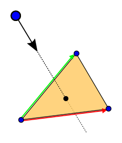
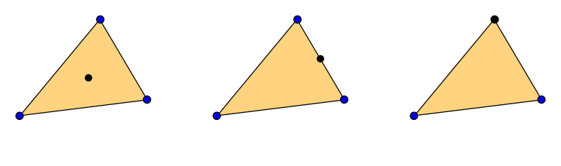
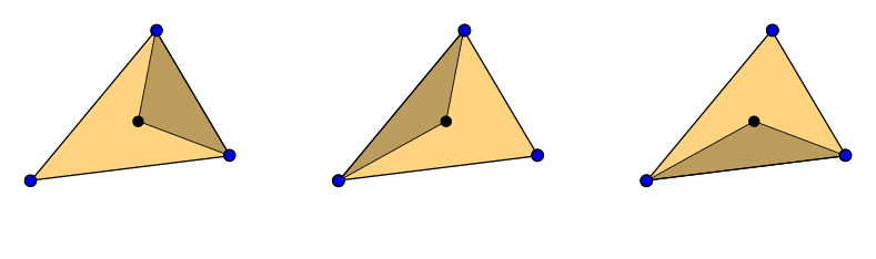
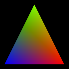
hitAttributeEXT vec2 baryCoord" Variable
vec3 barys = vec3(1.0f - baryCoord.x - baryCoord.y, baryCoord.x, baryCoord.y);
vec3 interpColor = blue * barys.x + red * barys.y + green * barys.z;
struct HitAttributeType {
vec3 normal;
vec2 texCoord;
vec2 baryCoord;
}; // type of the "hit" variable
...
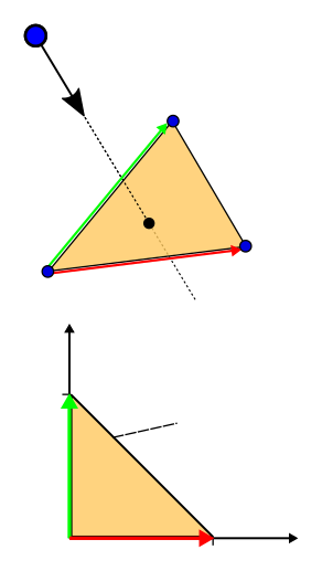
void main() { /**** INTERSECTION SHADER ****/
// ray-triangle intersection
// Note: Ray-triangle intersection is a
// built-in feature of the ray tracing shader pipeline.
// It is just provided for educational purpose.
// get bounding box in object space
vec3 aabbMin;
vec3 aabbMax;
gsnGetIntersectionBox(gl_InstanceID, gl_PrimitiveID, aabbMin, aabbMax);
vec3 diff = aabbMax - aabbMin;
// a, b, and c are the three triangle vertices
vec3 a = aabbMin + vec3(0.0, 0.0, diff.z / 2.0);
vec3 b = aabbMin + vec3(diff.x, 0.0, diff.z / 2.0);
vec3 c = aabbMin + vec3(diff.x / 2.0, diff.y, diff.z / 2.0);
// performing ray-triangle intersection in object space using
// Tomas Möller and Ben Trumbore:
// "Fast, Minimum Storage Ray / Triangle Intersection",
// Journal of Graphics Tools, 2(1):21--28, 1997
// here we use exactly the notation from the lecture slides
vec3 i = b - a;
vec3 j = c - a;
vec3 k = gl_ObjectRayOriginEXT - a;
vec3 r = gl_ObjectRayDirectionEXT;
// implementing ray/triangle intersection according to
// the lecture slides by computing
// (t, u, v) = (1 / (r x j) * i) ((k x i) * j, (r x j) *k, (k x i) * r)
vec3 rxj = cross(r, j);
float rxji = dot(rxj, i);
// denominator close to zero?
if (abs(rxji) < 1e-16) return;
uint hitKind = 0xFEu; // front facing
if (rxji < 0.0) {
hitKind = 0xFFu; // back facing
}
float f = 1.0f / rxji;
// compute u
float u = dot(rxj, k) * f;
if (u < 0.0f || u > 1.0f) return;
// compute v
vec3 kxi = cross(k, i);
float v = dot(kxi, r) * f;
if (v < 0.0 || v > 1.0) return;
if(u + v > 1.0) return;
// compute t
float t = dot(kxi, j) * f;
if (t < gl_RayTminEXT) return;
if (t > gl_RayTmaxEXT) return;
vec3 hitPoint = gl_ObjectRayOriginEXT + t * gl_ObjectRayDirectionEXT;
hit.texCoord = (hitPoint.xy - aabbMin.xy) / diff.xy;
hit.normal = vec3(0.0, 0.0, 1.0);
hit.baryCoord = vec2(u, v);
reportIntersectionEXT(t, hitKind);
}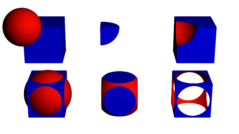
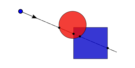
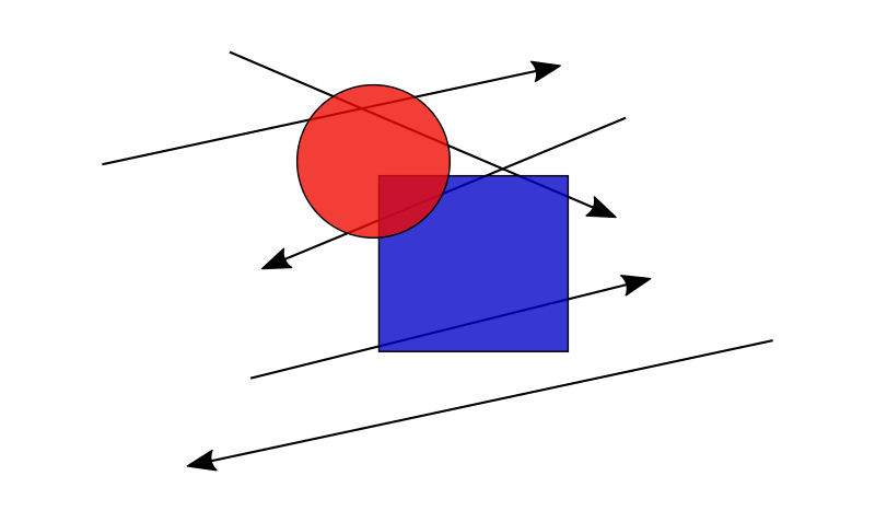
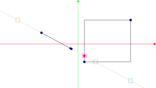
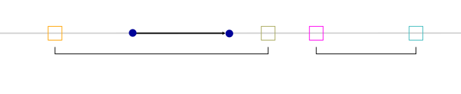
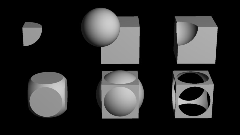
bool computeCsgUnion(in vec2 interval0, in vec2 interval1, float tmin,
                     out vec2 combinedInterval, out ivec2 hitIndex) {
  // handle the 5 cases from the lecture/tutorial
  if(interval0.x > interval0.y && interval1.x > interval1.y) {
    // case 1: no intersection
    combinedInterval = vec2(1e8, -1e8);
    return false;
  } else if(interval0.x <= interval0.y && interval1.x > interval1.y) {
     // case 2: only object0
    hitIndex =  ivec2(0, 0); // hit object0
    combinedInterval = interval0;
  } else if(interval0.x > interval0.y && interval1.x <= interval1.y) {
    // case 3: only object1
    hitIndex = ivec2(1, 1); // hit object1
    combinedInterval = interval1;
  } else if(!intervalsOverlap(interval0, interval1)) {
    //case 4: intervals are not overlaping
    if(interval0.x < interval1.x && interval0.y >= tmin) {
      combinedInterval = interval0;
      hitIndex = ivec2(0, 0); // hit object0
    } else if(interval1.y >= tmin) {
      combinedInterval = interval1;
      hitIndex = ivec2(1, 1); // hit object1
    } else {
      combinedInterval = vec2(1e8, -1e8);
      return false;
    }
  } else {
    //case 5: intervals are overlaping
    if(interval0.x < interval1.x) {
      hitIndex.x = 0; // hit object0
      combinedInterval.x = interval0.x;
    } else {
      hitIndex.x = 1; // hit object1
      combinedInterval.x = interval1.x;
    }
    if(interval0.y > interval1.y) {
      hitIndex.y = 0; // hit object0
      combinedInterval.y = interval0.y;
    } else {
      hitIndex.y = 1; // hit object1
      combinedInterval.y = interval1.y;
    }
  }
  return true;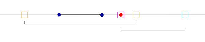
}bool computeCsgIntersection(in vec2 interval0, in vec2 interval1, float tmin,
out vec2 combinedInterval, out ivec2 hitIndex) {
// handle the 5 cases from the lecture/tutorial
if(interval0.x > interval0.y && interval1.x > interval1.y) {
// case 1: no intersection
combinedInterval = vec2(1e8, -1e8);
return false;
} else if(interval0.x <= interval0.y && interval1.x > interval1.y) {
// case 2: only object0
combinedInterval = vec2(1e8, -1e8);
return false;
} else if(interval0.x > interval0.y && interval1.x <= interval1.y) {
// case 3: only object1
combinedInterval = vec2(1e8, -1e8);
return false;
} else if(!intervalsOverlap(interval0, interval1)) {
//case 4: intervals are not overlaping
combinedInterval = vec2(1e8, -1e8);
return false;
} else {
//case 5: intervals are overlaping
if(interval0.x >= interval1.x) {
hitIndex.x = 0; // hit object0
combinedInterval.x = interval0.x;
} else {
hitIndex.x = 1; // hit object1
combinedInterval.x = interval1.x;
}
if(interval0.y <= interval1.y) {
hitIndex.y = 0; // hit object0
combinedInterval.y = interval0.y;
} else {
hitIndex.y = 1; // hit object1
combinedInterval.y = interval1.y;
}
}
return true;
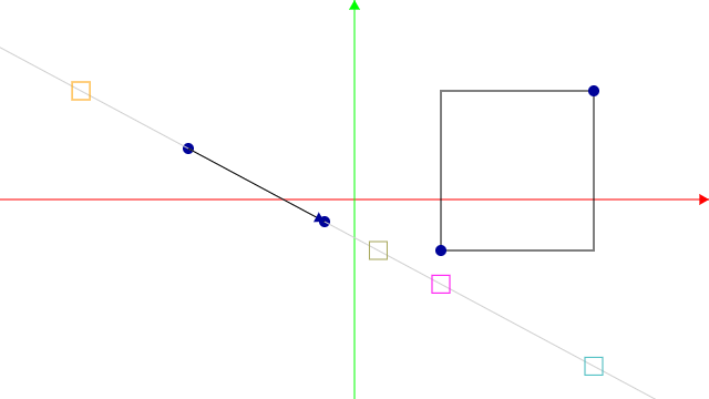
}bool computeCsgDifference(in vec2 interval0, in vec2 interval1, float tmin,
out vec2 combinedInterval, out ivec2 hitIndex) {
// handle the 5 cases from the lecture/tutorial
if(interval0.x > interval0.y && interval1.x > interval1.y) {
// case 1: no intersection
combinedInterval = vec2(1e8, -1e8);
return false;
} else if(interval0.x <= interval0.y && interval1.x > interval1.y) {
// case 2: only object0
hitIndex = ivec2(0, 0); // hit object0
combinedInterval = interval0;
} else if(interval0.x > interval0.y && interval1.x <= interval1.y) {
// case 3: only object1
combinedInterval = vec2(1e8, -1e8);
return false;
} else if(!intervalsOverlap(interval0, interval1)) {
//case 4: intervals are not overlaping
combinedInterval = interval0;
hitIndex = ivec2(0, 0); // hit object0
} else {
//case 5: intervals are overlaping
if(interval0.x < interval1.x && interval1.x >= tmin) {
hitIndex = ivec2(0, 1); // first hit object0, second hit object1
combinedInterval.x = interval0.x;
combinedInterval.y = interval1.x;
} else if(interval1.y < interval0.y && interval0.y >= tmin) {
hitIndex = ivec2(1, 0); // first hit object2, second hit object0
combinedInterval.x = interval1.y;
combinedInterval.y = interval0.y;
} else {
combinedInterval = vec2(1e8, -1e8);
return false;
}
}
return true;
}

Anregungen oder Verbesserungsvorschläge können auch gerne per E-Mail an mich gesendet werden: Kontakt