Image Synthesis
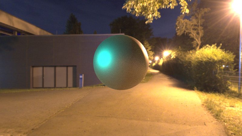
Image-based Lighting
Thorsten Thormählen
June 18, 2026
Part 3, Chapter 4
Thorsten Thormählen
June 18, 2026
Part 3, Chapter 4
This is the print version of the slides.
Advance slides with the → key or
by clicking on the right border of the slide
Slides can also be advanced by clicking on the left or right border of the slide.
| Type | Font | Examples |
|---|---|---|
| Variables (scalars) | italics | $a, b, x, y$ |
| Functions | upright | $\mathrm{f}, \mathrm{g}(x), \mathrm{max}(x)$ |
| Vectors | bold, elements row-wise | $\mathbf{a}, \mathbf{b}= \begin{pmatrix}x\\y\end{pmatrix} = (x, y)^\top,$ $\mathbf{B}=(x, y, z)^\top$ |
| Matrices | Typewriter | $\mathtt{A}, \mathtt{B}= \begin{bmatrix}a & b\\c & d\end{bmatrix}$ |
| Sets | calligraphic | $\mathcal{A}, B=\{a, b\}, b \in \mathcal{B}$ |
| Number systems, Coordinate spaces | double-struck | $\mathbb{N}, \mathbb{Z}, \mathbb{R}^2, \mathbb{R}^3$ |
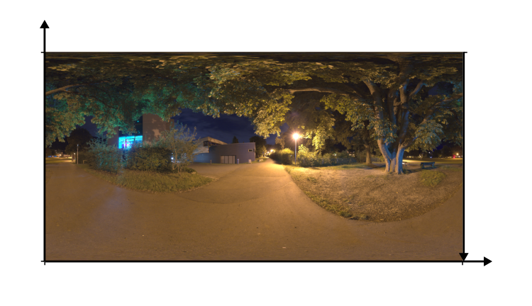
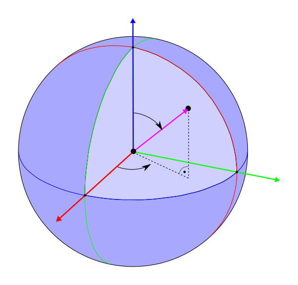
vec2 directionToSphericalEnvmap(vec3 dir) {
  float s = 0.5 - atan(dir.y, dir.x) / (2.0 * PI);
  float t = 1.0 / (PI) * acos(-dir.z);
  return vec2(s, t);
}
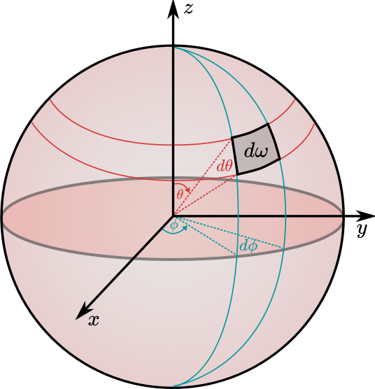
$\begin{align}\phi &= 2\pi \,(0.5 - s) \\ \theta &= \pi \, (1.0 - t) \end{align}$
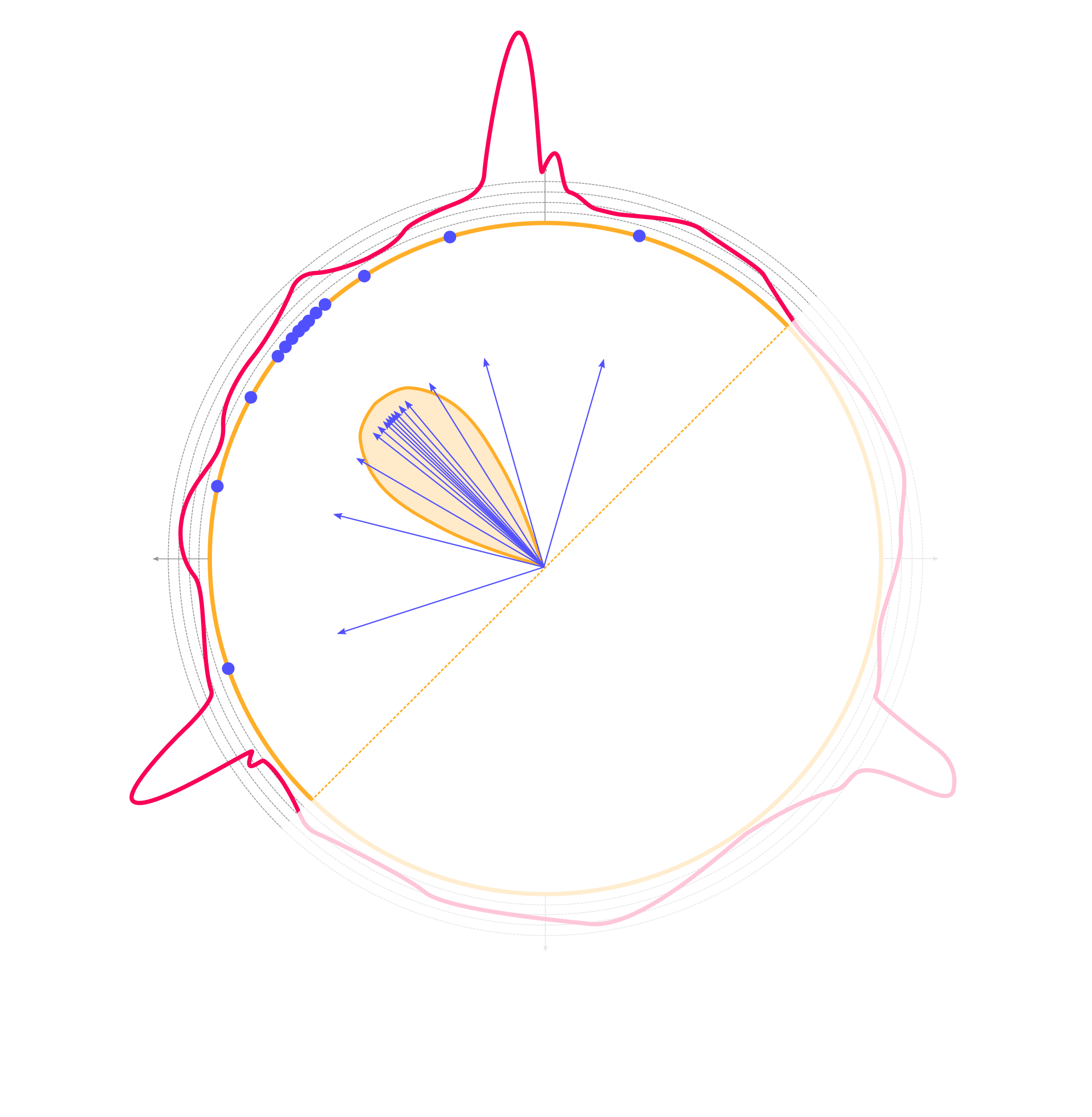
vec2 sampleEnvmap(sampler2D envmap, sampler2D rowAvg,
        float totalAvg, vec2 random) {

  ivec2 texSize = textureSize(rowAvg, 0);
  float sumY = 0.0;
  float prevSumY = 0.0;
  float ra = 1.0;
  int y = 0;
  for(y = 0; y < texSize.y; y++) {
    ra = texelFetch(rowAvg, ivec2(0, y), 0).r;
    float pt = ra / totalAvg;
    sumY += pt / float(texSize.y);
    if(sumY >= random.y) {
      break;
    }
    prevSumY = sumY;
  }
  float subPixelY = (random.y - prevSumY) / (sumY - prevSumY);

  ivec2 envSize = textureSize(envmap, 0);
  float sumX = 0.0;
  float prevSumX = 0.0;
  int xx = 0;
  for(xx= 0; xx < envSize.x; xx++) {
    vec3 rgb = pow(texelFetch(envmap, ivec2(xx, y), 0).rgb, vec3(2.2));
    float gray = dot(vec3(0.2989, 0.5866, 0.1145), rgb);
    float ps = gray / ra;
    sumX += ps / float(envSize.x);
    if(sumX >= random.x) {
      break;
    }
    prevSumX = sumX;
  }
  float subPixelX = (random.x - prevSumX) / (sumX - prevSumX);

  return vec2((float(xx) + subPixelX) / float(envSize.x),
              (float(y) + subPixelY) / float(texSize.y));
}
Please notify me by e-mail if you have questions, suggestions for improvement, or found typos: Contact