Multimedia Signal Processing
Convolution and Impulse Response
Thorsten Thormählen
May 04, 2026
Part 3, Chapter 1
Thorsten Thormählen
May 04, 2026
Part 3, Chapter 1
This is the print version of the slides.
Advance slides with the → key or
by clicking on the right border of the slide
Slides can also be advanced by clicking on the left or right border of the slide.
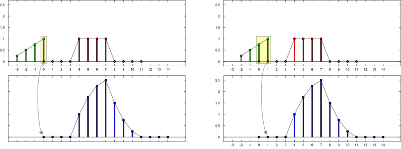
$\mathrm{f}[n] = \sum\limits_{k = -\infty}^{\infty} \mathrm{a}[k] \, \,\mathrm{b}[n-k]$
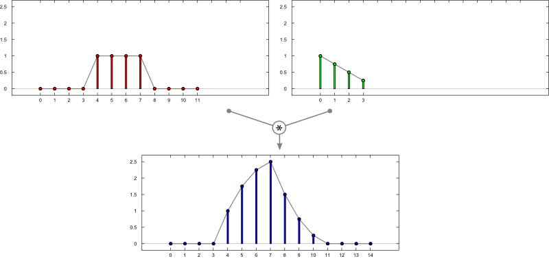
$\mathrm{f}[n] = \sum\limits_{k = -\infty}^{\infty} \mathrm{a}[k] \, \,\mathrm{b}[n-k]$
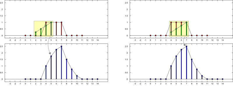
Konstruktion:
$\mathrm{f}[n] = \sum\limits_{k = -\infty}^{\infty} \mathrm{a}[k] \, \,\mathrm{b}[n-k]$
Konstruktion:


Please notify me by e-mail if you have questions, suggestions for improvement, or found typos: Contact