Multimedia Signal Processing
Frequency Transforms

• Time-discrete frequency transforms represent a time-varying signal $\mathrm{f}[n]$ with $n \in \mathbb{Z}$ as a superposition of basis functions $\mathrm{b}_u[n]$ that have a locality in the frequency domain
  $\mathrm{f}[n] = \sum\limits_u \mathrm{F}[u] \, \mathrm{b}_u[n]$
• The coefficients $\mathrm{F}[u]$ of the basis functions are, therefore, a representation of the time-varying signal $\mathrm{f}[n]$ in the frequency domain (i.e., in the space spanned by the basis functions).
• By the mapping $\mathrm{f}[n] \mapsto \mathrm{F}[u]$, the transformation from the time domain to the frequency domain is performed
• By the mapping $\mathrm{F}[u] \mapsto \mathrm{f}[n]$, the transformation from the frequency domain to the time domain is performed

• Examples of discrete frequency transforms are
  • Discrete Fourier Transform (DFT)
  • Discrete Cosine Transform (DCT)
  • Discrete Wavelet Transform (DWT)

• The discrete Fourier transform (DFT) for a complex periodic signal $\mathrm{f}[n]$ of period length $N$ is calculated by:
  $\mathrm{F}[u] = \sum\limits_{n=0}^{N-1} \mathrm{f}[n] \, e^{-2 \pi i \frac{n\, u}{N} } \quad \quad \forall \, \, u \in [0;N-1]$
• The inverse discrete Fourier transform (IDFT) is defined as
  $\mathrm{f}[n] = \frac{1}{N} \sum\limits_{u=0}^{N-1} \mathrm{F}[u] \, e^{2 \pi i \, \frac{n\, u}{N} } \quad \quad \forall \, \, n \in [0;N-1]$
• Thus, the basis functions used in the inverse Fourier transform are:
  $\begin{array}{ll} \mathrm{b}_u[n] &= \frac{1}{N} e^{2 \pi i \frac{n\, u}{N} } \\ &= \frac{1}{N} \cos\left(2 \pi \frac{n\, u}{N} \right) + i\, \frac{1}{N} \sin\left(2 \pi \frac{n\, u}{N} \right) \end{array} $
  i.e., the basis functions are complex functions with the
  imaginary unit $i = \sqrt{-1}$

• In total, there are N different basis functions:
  $\mathrm{b}_u[n] = \frac{1}{N} \cos\left(2 \pi \frac{n\, u}{N} \right) + i\, \frac{1}{N} \sin\left(2 \pi \frac{n\, u}{N} \right)$
  • For $\mathrm{b}_0[n]$, the real and imaginary part is constant
  • For $\mathrm{b}_1[n]$, the wavelength of the cosine and the sine wave corresponds to the period length of the input signal
  • For increasing $u$, the wavelength is halved in each instance (or the frequency doubled)

• Presentation of the basic functions
  $\mathrm{b}_u[n] = \frac{1}{N} \cos\left(2 \pi \frac{n\, u}{N} \right) + i\, \frac{1}{N} \sin\left(2 \pi \frac{n\, u}{N} \right)$
  for $N=32$:

Real part

Imaginary part

$b_0$

$b_1$

$b_2$

$b_3$

$n$

• Presentation of the basic functions
  $\mathrm{b}_u[n] = \frac{1}{N} \cos\left(2 \pi \frac{n\, u}{N} \right) + i\, \frac{1}{N} \sin\left(2 \pi \frac{n\, u}{N} \right)$
  for $N=32$:

Real part

Imaginary part

$b_1$

$b_{16}$

$b_{30}$

$b_{31}$

$n$

• Observations:
  • Although the frequency is actually doubled for each increase in $u$, the observed frequency of the oscillation does not continue to increase for $u > N/2$ because of discrete-time sampling
  • Instead, the observed frequency decreases. It holds:
    $\operatorname{Re}(\mathrm{b}_u[n]) = \operatorname{Re}(\mathrm{b}_{N-u}[n])$ und $\operatorname{Im}(\mathrm{b}_u[n]) = -\operatorname{Im}(\mathrm{b}_{N-u}[n])$
  • So the basis function with the highest frequency is $\mathrm{b}_{N/2}$
  • All basis functions for $N = 16$:
    

• Since the input signal and all basis functions are periodic in $N$, $\mathrm{F}[u]$ is also periodic in $N$
• In particular, it holds:
  $\mathrm{F}[N-u] = \mathrm{F}[-u] $
• By this mathematical reasoning, negative frequencies are now possible
• Negative frequencies do not exist physically. In the case of the DFT, it is only a mathematical way of describing the inverse direction of rotation in the complex plane
• If we mentally interpret frequencies larger than $u > N/2$ as negative frequencies, then this has the advantage that it corresponds to the observation that the basis function $\mathrm{b}_{N/2}$ has the highest frequency
  

• Besides the use of negative frequencies it is also common to represent real and imaginary part of $\mathrm{F}[u]$ by magnitude and phase
• The magnitude is calculated by:
  $\mathrm{b}[u] = \sqrt{\operatorname{Re}(\mathrm{F}[u])^2 + \operatorname{Im}(\mathrm{F}[u])^2}$
• The formula for the phase is:
  $\mathrm{\phi}[u] = \operatorname{atan2}(\operatorname{Im}(\mathrm{F}[u]),\operatorname{Re}(\mathrm{F}[u]))$

$\operatorname{Im}(\mathrm{F}[u])$

$\operatorname{Re}(\mathrm{F}[u])$

$\phi$

$sin(\phi)$

$cos(\phi)$

$\begin{array}{ll} \mathrm{F}[u] &= \sum\limits_{u=0}^{N-1} \mathrm{f}[n] \, e^{-2 \pi i \frac{n\, u}{N} } \\ &= \sum\limits_{u=0}^{N-1} \mathrm{f}[n]\left( \cos\left(- 2 \pi \frac{n\, u}{N} \right) + i\, \sin\left(- 2 \pi \frac{n\, u}{N} \right) \right)\\ &= \sum\limits_{u=0}^{N-1} \mathrm{f}[n]\left( \cos\left(2 \pi \frac{n\, u}{N} \right) - i\, \sin\left(2 \pi \frac{n\, u}{N} \right) \right)\\ &= \sum\limits_{u=0}^{N-1} \left(\operatorname{Re}(\mathrm{f}[n]) + i\, \operatorname{Im}(\mathrm{f}[n])\right) \left( \cos\left(2 \pi \frac{n\, u}{N} \right) - i\, \sin\left(2 \pi \frac{n\, u}{N} \right) \right) \\ \operatorname{Re}(\mathrm{F}[u]) &= \sum\limits_{u=0}^{N-1} \operatorname{Re}(\mathrm{f}[n]) \cos\left(2 \pi \frac{n\, u}{N} \right) + \operatorname{Im}(\mathrm{f}[n]) \sin\left(2 \pi \frac{n\, u}{N} \right) \\ \operatorname{Im}(\mathrm{F}[u]) &= \sum\limits_{u=0}^{N-1} \operatorname{Im}(\mathrm{f}[n]) \cos\left(2 \pi \frac{n\, u}{N} \right) - \operatorname{Re}(\mathrm{f}[n]) \sin\left(2 \pi \frac{n\, u}{N} \right) \\ \end{array} $

$\begin{array}{ll} \mathrm{f}[n] &= \frac{1}{N} \sum\limits_{u=0}^{N-1} \mathrm{F}[u] \, e^{2 \pi i \frac{n\, u}{N} } \\ &= \frac{1}{N} \sum\limits_{u=0}^{N-1} \mathrm{F}[u]\left( \cos\left(2 \pi \frac{n\, u}{N} \right) + i\, \sin\left(2 \pi \frac{n\, u}{N} \right) \right)\\ &= \frac{1}{N} \sum\limits_{u=0}^{N-1} \left(\operatorname{Re}(\mathrm{F}[u]) + i\, \operatorname{Im}(\mathrm{F}[u])\right) \left( \cos\left(2 \pi \frac{n\, u}{N} \right) + i\, \sin\left(2 \pi \frac{n\, u}{N} \right) \right) \\ \operatorname{Re}(\mathrm{f}[n]) &= \frac{1}{N} \sum\limits_{u=0}^{N-1} \operatorname{Re}(\mathrm{F}[u]) \cos\left(2 \pi \frac{n\, u}{N} \right) - \operatorname{Im}(\mathrm{F}[u]) \sin\left(2 \pi \frac{n\, u}{N} \right) \\ \operatorname{Im}(\mathrm{f}[n]) &= \frac{1}{N} \sum\limits_{u=0}^{N-1} \operatorname{Im}(\mathrm{F}[u]) \cos\left(2 \pi \frac{n\, u}{N} \right) + \operatorname{Re}(\mathrm{F}[u]) \sin\left(2 \pi \frac{n\, u}{N} \right) \\ \end{array} $

• For the real part of $\mathrm{f}[n]$, the cosine components are represented by the coefficients in the real part of $\mathrm{F}[u]$, and the sine components by the coefficients in the imaginary part
• For the imaginary part of $\mathrm{f}[n]$, this is the other way around

• For a real periodic signal $\mathrm{f}[n]$, the calculation of the real and imaginary part of $\mathrm{F}[u]$ can be done completely independently from each other:
  $\operatorname{Re}(\mathrm{F}[u]) = \sum\limits_{n=0}^{N-1} \mathrm{f}[n] \, \cos(2 \pi \frac{n\, u}{N}) \quad$ and $\quad \operatorname{Im}(\mathrm{F}[u]) = -\sum\limits_{n=0}^{N-1} \mathrm{f}[n] \, \sin(2 \pi \frac{n\, u}{N})$
• Due to the symmetry of the basis functions, it follows:
  $\operatorname{Re}(\mathrm{F}[u]) = \operatorname{Re}(\mathrm{F}[N-u])\quad$ and $\quad\operatorname{Im}(\mathrm{F}[u]) = -\operatorname{Im}(\mathrm{F}[N-u])$
• I.e., for a real signal $\mathrm{f}[n]$ only the coefficients $\mathrm{F}[u]$ for $0 \le u \le N/2$ have to be calculated and stored
• In this case, the inverse transform is given by::
  $\mathrm{f}[n] = \frac{1}{N} \sum\limits_{u=0}^{N/2} \mathrm{w}[u] \left(\operatorname{Re}(\mathrm{F}[u]) \cos\left(2 \pi \frac{n\, u}{N} \right) - \operatorname{Im}(\mathrm{F}[u]) \sin\left(2 \pi \frac{n\, u}{N} \right) \right)$
  where all summands are weighted twice except for $u=0$ and $u=N/2$:
  $\mathrm{w}[u] = \begin{cases} 1 & \,\,:\,\, u = 0 \lor u=N/2\\ 2 & \,\,:\,\, u \ne 0 \land u \ne N/2 \end{cases}$

• Linearity:
  $a_1 \mathrm{f}_1[n] + a_2 \, \mathrm{f}_2[n] \quad \stackrel{\operatorname{dft}}{\longrightarrow} \quad a_1 \mathrm{F}_1[u] + a_2 \, \mathrm{F}_2[u]$
• Average value:
  $ \frac{1}{N} \sum\limits_{n=0}^{N-1} \mathrm{f}[n] = \frac{1}{N} F(0)$
• Reciprocity of the time domain and the frequency domain:
  $\begin{array}{ll} f[n] \quad &\stackrel{\operatorname{dft}}{\longrightarrow}& \quad F[u]\\ F[n] \quad &\stackrel{\operatorname{dft}}{\longrightarrow}& \quad N \, f[u] \end{array}$

• Shift in the time domain:
  $f[n-n_0] \quad \stackrel{\operatorname{dft}}{\longrightarrow} \quad \mathrm{F}[u] \, e^{-2 \pi i \frac{n_0 u}{N} }$
• Shift in the frequency domain:
  $\mathrm{f}[n]\, e^{2 \pi i \frac{n u_0}{N} } \quad \stackrel{\operatorname{dft}}{\longrightarrow} \quad F(u-u_0)$
• A convolution in the time domain corresponds to a multiplication in the frequency domain:
  $f_1[n] \ast f_2[n] \quad \stackrel{\operatorname{dft}}{\longrightarrow} \quad F_1[u] \, F_2[u]$
• A convolution in the frequency domain corresponds to a multiplication in the time domain:
  $f_1[n] \, f_2[n] \quad \stackrel{\operatorname{dft}}{\longrightarrow} \quad \frac{1}{N} F_1[u] \ast F_2[u]$

• For any real signal $\mathrm{f}[n]$, the real part of the DFT is symmetric, and the imaginary part is anti-symmetric:
  $\operatorname{Re}(\mathrm{F}[u]) = \operatorname{Re}(\mathrm{F}[N-u])$ and $\operatorname{Im}(\mathrm{F}[u]) = -\operatorname{Im}(\mathrm{F}[N-u])$
• If a real signal $\mathrm{f}[n]$ is symmetric, i.e.
  $\mathrm{f}[n] = f[N-n]$ or resp. $\mathrm{f}[n] = f[-n]$
  then $\operatorname{Im}(\mathrm{F}[u]) = 0$
• If a real signal $\mathrm{f}[n]$ is anti-symmetric, i.e.
  $\mathrm{f}[n] = -f[N-n]$ or resp. $\mathrm{f}[n] = -f[-n]$
  then $\operatorname{Re}(\mathrm{F}[u]) = 0$

$\mathrm{f}[n] = \cos\left(2 \pi \frac{n\, u_0}{N} \right), \quad n \in [0; N-1]$

$\mathrm{F}[u] =\,\frac{N}{2} \delta(u-u_0) + \frac{N}{2} \delta(u-(N-u_0)), \quad u \in [0; N-1]$

Mathematical verification:
$\begin{array}{ll} \operatorname{Re}(\mathrm{f}[n]) &= \frac{1}{N} \sum\limits_{u=0}^{N-1} \operatorname{Re}(\mathrm{F}[u]) \cos\left(2 \pi \frac{n\, u}{N} \right) - \operatorname{Im}(\mathrm{F}[u]) \sin\left(2 \pi \frac{n\, u}{N} \right) \\ &= \frac{1}{N} \sum\limits_{u=0}^{N-1} \frac{N}{2} \delta(u-u_0) + \frac{N}{2} \delta(u-(N-u_0)) \cos\left(2 \pi \frac{n\, u}{N} \right) \\ &= \frac{1}{2} \cos\left(2 \pi \frac{n\, u_0}{N} \right) + \frac{1}{2} \cos\left(2 \pi \frac{n\, (N-u_0)}{N} \right) = \cos\left(2 \pi \frac{n\, u_0}{N}\right)\\ \operatorname{Im}(\mathrm{f}[n]) &= \frac{1}{N} \sum\limits_{u=0}^{N-1} \operatorname{Im}(\mathrm{F}[u]) \cos\left(2 \pi \frac{n\, u}{N} \right) + \operatorname{Re}(\mathrm{F}[u]) \sin\left(2 \pi \frac{n\, u}{N} \right) \\ &= \frac{1}{2} \sin\left(2 \pi \frac{n\, u_0}{N} \right) + \frac{1}{2} \sin\left(2 \pi \frac{n\, (N-u_0)}{N} \right) = 0\\ \end{array} $

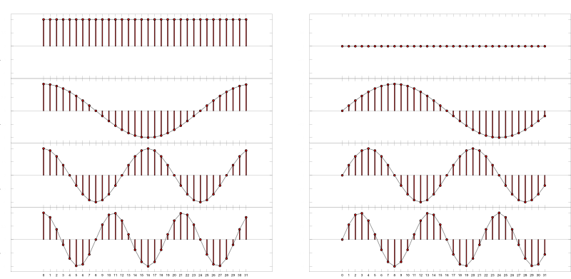
$\mathrm{f}[n] = \cos\left(2 \pi \frac{n\, u_0}{N} \right), \quad n \in [0; N-1]$

$\mathrm{F}[u] =\,\frac{N}{2} \delta(u-u_0) + \frac{N}{2} \delta(u-(N-u_0)), \quad u \in [0; N-1]$

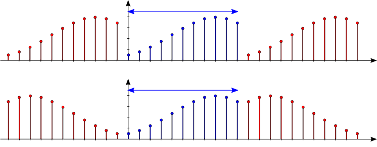
Graphical visualization for $N =16$ and $u_0 = 3$:

$\operatorname{Re}(\mathrm{f}[n])$

$\operatorname{Im}(\mathrm{f}[n])$

$\operatorname{Re}(\mathrm{f}[n])$

$\operatorname{Im}(\mathrm{f}[n])$

$\operatorname{Re}(\mathrm{F}[u])$

$\operatorname{Im}(\mathrm{F}[u])$

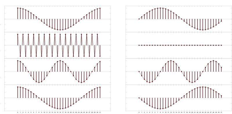
$\mathrm{f}[n] = \sin\left(2 \pi \frac{n\, u_0}{N} \right), \quad n \in [0; N-1]$

$\mathrm{F}[u] =\,i \, \frac{N}{2} \left( -\delta(u-u_0) + \delta(u-(N-u_0))\right), \quad u \in [0; N-1]$

Graphical visualization for $N =16$ und $u_0 = 3$:

$\operatorname{Re}(\mathrm{f}[n])$

$\operatorname{Im}(\mathrm{f}[n])$

$\operatorname{Re}(\mathrm{f}[n])$

$\operatorname{Im}(\mathrm{f}[n])$

$\operatorname{Re}(\mathrm{F}[u])$

$\operatorname{Im}(\mathrm{F}[u])$

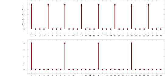
$\mathrm{f}[n] = \cos\left(2 \pi \frac{n\, u_1}{N} \right) + \sin\left(2 \pi \frac{n\, u_2}{N} \right), \quad n \in [0; N-1]$

$\mathrm{F}[u] = {\small \frac{N}{2} \delta(u-u_1) + \frac{N}{2} \delta(u-(N-u_1)) - \frac{iN}{2} \, \delta(u-u_2) + \frac{iN}{2} \delta(u-(N-u_2))}$

Graphical visualization for $N =16$, $u_1 = 1$ and $u_2 = 3$:

$\operatorname{Re}(\mathrm{f}[n])$

$\operatorname{Im}(\mathrm{f}[n])$

$\operatorname{Re}(\mathrm{f}[n])$

$\operatorname{Im}(\mathrm{f}[n])$

$\operatorname{Re}(\mathrm{F}[u])$

$\operatorname{Im}(\mathrm{F}[u])$

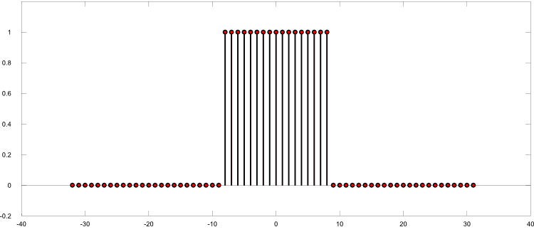
$\mathrm{f}[n] = \cos\left(2 \pi \frac{n\, u_0}{N} \right) + i\,\sin\left(2 \pi \frac{n\, u_0}{N} \right), \quad n \in [0; N-1]$

$\mathrm{F}[u] =\, N \, \delta(u-u_0)$

Graphical visualization for $N =16$ and $u_0 = 4$:

$\operatorname{Re}(\mathrm{f}[n])$

$\operatorname{Im}(\mathrm{f}[n])$

$\operatorname{Re}(\mathrm{f}[n])$

$\operatorname{Im}(\mathrm{f}[n])$

$\operatorname{Re}(\mathrm{F}[u])$

$\operatorname{Im}(\mathrm{F}[u])$

• Unit impulse
  $\mathrm{f}[n] = \delta[n] \quad n \in [0; N-1]$
  $\mathrm{F}[u] = 1, \quad u \in [0; N-1]$
• Constant function
  $\mathrm{f}[n] = A, \quad n \in [0; N-1]$
  $\mathrm{F}[u] = N \, A\,\delta[n], \quad u \in [0; N-1]$
• Gaussian function
  $\mathrm{f}[n] = \frac{1}{\sigma \sqrt{2\pi}} \exp\left(\frac{n^2}{2 \, \sigma^2}\right) \quad n \in [0; N-1]$
  $\mathrm{F}[u] = \exp\Big(\frac{u^2}{2 \, (1 / \sigma)^2}\Big) \quad u \in [0; N-1]$

• $K$ unit impulses at a distance $P$ (i.e., signal length is $N=K\,P$ ) :
  $\mathrm{f}[n] = \sum\limits_{k=0}^{K-1} \delta[n - k\,P]$
  yields a DFT consisting of $P$ unit impulses at a distance $K$
  $\mathrm{F}[u] = K\,\sum\limits_{p=0}^{P-1} \delta[u - p\,K]$
• Example: $K=8$ und $P=4$

$\mathrm{f}[n]$

$\mathrm{F}[u]$

• A discrete-time rectangular pulse with the pulse width $P$:
  $\mathrm{f}[n] = \begin{cases} 1 & \,\,:\,\, |f| < P/2 \\ 0.5 & \,\,:\,\, |f| = P/2 \\ 0 & \,\,:\,\, |f| > P/2 \\ \end{cases}$
• The figure shows a rectangular pulse with a pulse width $P=17$ and length $N=64$

$\mathrm{f}[n]$

$n$

• To apply the DFT, $n$ must be in the range $[0; N-1]$
• Therefore, we first shift the negative part to the right by $N = 64$
• This is allowed because the input signal of the DFT must be periodic in $N$

$\mathrm{f}[n]$

$n$

• The DFT of the rectangular pulse is
  $\operatorname{Re}(\mathrm{F}[u]) = \frac{\sin(\pi u P / N)}{\pi u / N}$
• I.e., it has the general shape of a sinc function
  $\operatorname{sinc}(x) = \frac{\sin(\pi x)}{\pi x}$

$\operatorname{Re}(\mathrm{F}[u])$

$u$

• The discrete cosine transform (DCT) for a real signal $\mathrm{f}[n]$ of length $N$ is calculated by:
  $\mathrm{F}[u] = \sum\limits_{n=0}^{N-1} \mathrm{w}[u]\, \mathrm{f}[n] \, \cos(\frac{\pi}{N} \, (n + 0.5) \, u ) \quad \quad \forall \, \, u \in [0;N-1]$
  with
  $\mathrm{w}[u] = \begin{cases} 1.0 / \sqrt{N} & \,\,:\,\, u = 0 \\ \sqrt{2/N} & \,\,:\,\, u \ne 0 \end{cases}$
• The corresponding inverse discrete cosine transform (IDCT) is:
  $\mathrm{f}[n] = \sum\limits_{u=0}^{N-1} \mathrm{w}[u]\, \mathrm{F}[u] \, \cos(\frac{\pi}{N} \, (u + 0.5) \, n ) \quad \quad \forall \, \, n \in [0;N-1]$

• Instead of a combination of sine and cosine functions, as in DFT, the DCT uses only cosine waves as basis functions
  $\mathrm{b}_u[n] = \cos(\frac{\pi}{N} \, (n + 0.5) \, u )$
• These are cosine functions that are shifted to the left by half a sample value
• In contrast to the DFT, where the function is periodically extended during the reconstruction, the DCT extends the function symmetrically

DFT

DCT

$\mathrm{f}[n]$

$N$

$N$

• This means that there are fewer discontinuities at the boundaries, so that with the DCT the original signal can often be reconstructed with fewer coefficients than with the DFT
• Therefore, the DCT is often used in compression techniques, such as JPEG or MP3 (see later chapters)

• Example: Reconstruction of a signal $N=128$ with only $32$ DFT (or DCT) coefficients

DFT Reconstruction

DCT Reconstruction

Original