Control Keys

move to next slide (also Enter or Spacebar).
move to previous slide.
 d  enable/disable drawing on slides
 p  toggles between print and presentation view
CTRL  +  zoom in
CTRL  -  zoom out
CTRL  0  reset zoom

Slides can also be advanced by clicking on the left or right border of the slide.

Notation

Type Font Examples
Variables (scalars) italics $a, b, x, y$
Functions upright $\mathrm{f}, \mathrm{g}(x), \mathrm{max}(x)$
Vectors bold, elements row-wise $\mathbf{a}, \mathbf{b}= \begin{pmatrix}x\\y\end{pmatrix} = (x, y)^\top,$ $\mathbf{B}=(x, y, z)^\top$
Matrices Typewriter $\mathtt{A}, \mathtt{B}= \begin{bmatrix}a & b\\c & d\end{bmatrix}$
Sets calligraphic $\mathcal{A}, B=\{a, b\}, b \in \mathcal{B}$
Number systems, Coordinate spaces double-struck $\mathbb{N}, \mathbb{Z}, \mathbb{R}^2, \mathbb{R}^3$

Echo

  • A simple echo can be realized by weighted addition of the time-delayed original signal
    $\mathrm{y}[n] = \mathrm{x}[n] + A \, \mathrm{x}[n - d]$
  • Of course, several echoes can also be used
    $\mathrm{y}[n] = \mathrm{x}[n] + A_1 \, \mathrm{x}[n - d_1] + A_2 \, \mathrm{x}[n - d_2] + A_3 \, \mathrm{x}[n - d_3] + \dots$
  • This could also be realized with a convolution:
    $\mathrm{y}[n] = \mathrm{x}[n] \ast \mathrm{h}[n]$
    with $\mathrm{h}[n] = \delta[n] + A_1 \, \delta[n - d_1] + A_2 \, \delta[n - d_2] + A_3 \, \delta[n - d_3] + \dots$
  • echo
    $\mathrm{h}[n]$
    $d_1$
    $d_2$
    $d_3$
    $n$
    However, one disadvantage of convolution is that the calculation is quite inefficient for longer delays, as a large number of zeros need to be added up. For this reason, a direct implementation is generally faster.

Chorus

  • In the case of chorus, the signal is also combined with delayed copies, but the delay times are shorter compared to echo (approx. 10 to 40 ms)
  • In addition, the delay time is modulated with a sine wave
    $\mathrm{y}[n] = \mathrm{x}[n] + A_1 \, \mathrm{x}[n - (d_1 + e_1 \sin(2 \pi \,f_1)) ]$
  • Parameters: Delay time $d_1$, modulation depth $e_1$ and modulation frequency $f_1$
  • The sound becomes fuller and more vibrant
  • Example: Original
    With chorus: $d_1 = 40\,\mbox{ms}$, $e_1 = 2 \, \mbox{ms}$, $f_1 = 0.5 \, \mbox{Hz}$
Source: Extracted from F#120-AcousticImpro by Javolenus, CC-BY-NC

Filters with Feedback

Filters with Feedback

  • The filters considered so far could be implemented using convolution (albeit inefficiently). The output function $\mathrm{y}[n]$ was only dependent on the input function $\mathrm{x}[n]$ and the impulse response $\mathrm{h}[n]$
  • Now, a feedback of the already calculated output values is also allowed, i.e. $\mathrm{y}[n]$ can also be a function of $\mathrm{y}[n-1], \mathrm{y}[n-2], \mathrm{y}[n-3], \dots$

Filters without Feedback

  • Without Feedback
    $\mathrm{y}[n] = a_0 \, \mathrm{x}[n] \,\,+\,\, a_1 \, \mathrm{x}[n-1] \,\,+\,\, a_2 \, \mathrm{x}[n-2] \,\,+\,\, a_3 \, \mathrm{x}[n-3] \,\,+\,\, \dots$
fir_block
$\mathrm{x}[n]$
$\mathrm{y}[n]$
$a_n$
$a_{n-1}$
$a_2$
$a_1$
$a_0$

Filters with Feedback

  • With Feedback:
    $\begin{array}{rrrrr} \mathrm{y}[n] = a_0 \, \mathrm{x}[n] &+\,\, a_1 \, \mathrm{x}[n-1] &+\,\, a_2 \, \mathrm{x}[n-2] &+\,\, a_3 \, \mathrm{x}[n-3] &+\,\, \dots \\ &+\,\, b_1 \, \mathrm{y}[n-1] &+\,\, b_2 \, \mathrm{y}[n-2] &+\,\, b_3 \, \mathrm{y}[n-3] &+\,\, \dots \end{array}$
iir_block
$\mathrm{x}[n]$
$\mathrm{y}[n]$
$a_n$
$a_{n-1}$
$a_2$
$a_1$
$a_0$
$b_n$
$b_{n-1}$
$b_2$
$b_1$

Filters with Feedback

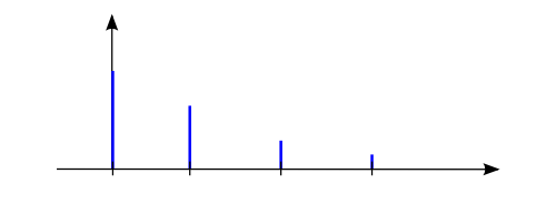
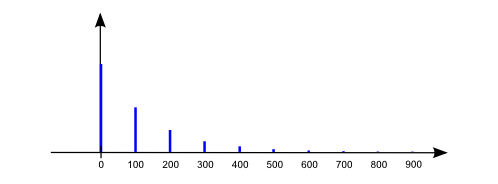
  • We consider the impulse response of a filter with feedback with $a_0 = 1$ and $b_{100} = 0.5$ and all other coefficients equal to zero
    irst_iir
    $\mathrm{h}[n]$
    $n$
  • This impulse response looks similar to the impulse response of the echo effect, which we were previously only able to generate using a very long convolution. With each additional echo, the convolution became longer and the computing time increased accordingly.
  • The filter with feedback generates many echoes, whereby only very few coefficients are required, which leads to a very low computation time
  • The echoes become smaller and smaller, but in principle the impulse response has an infinite length. This is why filters with feedback are also called IIR (infinite impulse response) filters and filters without feedback are called FIR (finite impulse response) filters

Comparison of FIR and IIR Filters

FIR Filters IIR Filters
More coefficients less coefficients
Higher computational effort Lower computational effort
Higher memory requirement Lower memory requirement
Always stable Possibly unstable
Rounding errors are not a problem Rounding errors may have a large effect due to feedback
Linear phase or zero phase is easy to realize Phase is distorted non-linearly

Reverb

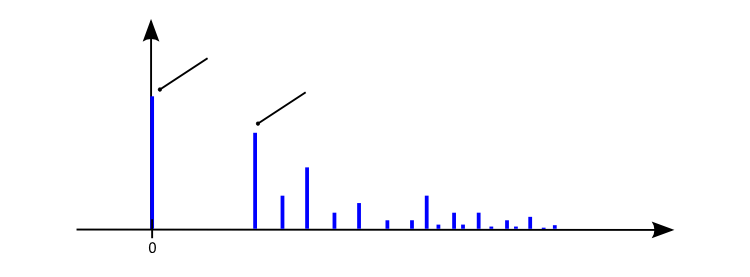
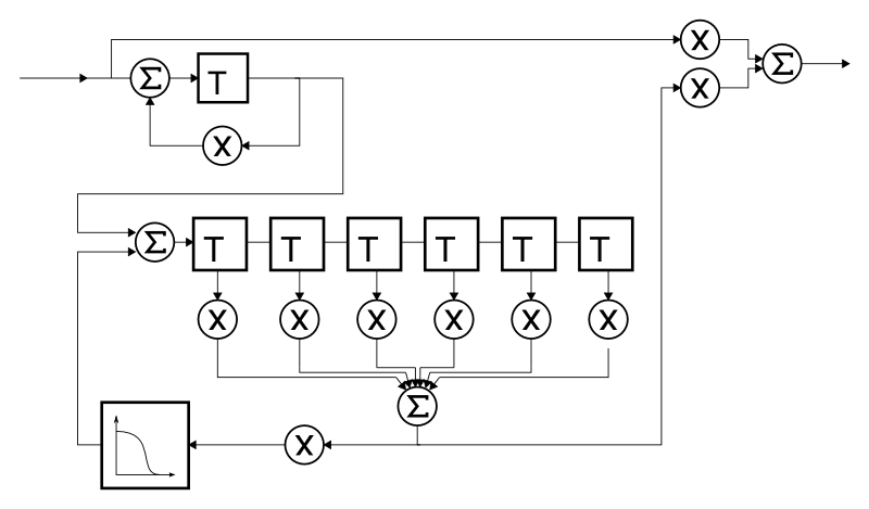
  • Reverb is caused by the reflection of the sound source on the walls of a room
  • Depending on the size of the room and the absorption properties of the walls, different impulse responses are generated
  • There is typically a delay until the first reflection occurs
  • This is followed by the diffuse reverb components
reverb
$\mathrm{h}[n]$
$n$
Original impulse
First reflection
diffuse reverb components

Reverb

reverb_schema
$t_1$
$t_{2a}$
$t_{2b}$
$t_{2c}$
$t_{2d}$
$t_{2e}$
$t_{2f}$
Low pass
Dry
Reverb
$\mathrm{x}[n]$
$\mathrm{y}[n]$
Feedback
Feedback
Source: based on P. Ackermann, Computer und Musik: Eine Einführung in die digitale Klang- und Musikverarbeitung, Springer, 1991, Page 137, Image 6.18

Non-linear Filters

Non-linear Filters

  • The previous filters were all describable by their impulse response, i.e. they were realized by LZI systems
  • We will now look at examples of non-linear systems

Overdrive

  • With overdrive, low amplitudes are amplified linearly, large amplitudes are limited to 1, with a smooth transition in between
    $\mathrm{y}[n] = \begin{cases} 2 \, \mathrm{x}[n] & \,\,:\,\, 0 \le \mathrm{x}[n] < 1/3 \\ \frac{3-(2-3 \, \mathrm{x}[n])^2}{3} & \,\,:\,\, 1/3 \le \mathrm{x}[n] < 2/3 \\ 1.0 & \,\,:\,\, 2/3 \le \mathrm{x}[n] \\ \end{cases}$
  • The original signal $\mathrm{x}_{\mathrm{in}}[n]$ is often linearly scaled with a gain factor $g$ before the overdrive is applied:
    $\mathrm{x}[n] = g \, \mathrm{x}_{\mathrm{in}}[n] $
Source: based on U. Zölzer, DAFX: Digital Audio Effects, Wiley, 2011, 2nd Edition

Distortion

  • With a distortion filter, the signal undergoes non-linear amplification
  • Lower amplitudes are amplified more than higher amplitudes, e.g. by:
    $\mathrm{y}[n] = \begin{cases} \frac{\mathrm{x}[n]}{|\mathrm{x}[n]|} \left( 1 - \exp\left(g \, |\mathrm{x}[n]| \right) \right) & \,\,:\,\, \mathrm{x}[n] \ne 0 \\ 0 & \,\,:\,\, \mathrm{x}[n] = 0 \end{cases}$
    whereby the effect becomes more pronounced the higher the gain factor $g$ is selected

Are there any questions?

questions

Please notify me by e-mail if you have questions, suggestions for improvement, or found typos: Contact

More lecture slides

Slides in German (Folien auf Deutsch)