Multimedia Signal Processing
Image Processing

Thorsten Thormählen
June 23, 2023
Part 6, Chapter 1

This is the print version of the slides.

Advance slides with the → key or
by clicking on the right border of the slide

Control Keys

→ move to next slide (also Enter or Spacebar).
← move to previous slide.
d enable/disable drawing on slides
p toggles between print and presentation view
CTRL + zoom in
CTRL - zoom out
CTRL 0 reset zoom

Slides can also be advanced by clicking on the left or right border of the slide.

Notation

Type	Font	Examples
Variables (scalars)	italics	$a, b, x, y$
Functions	upright	$\mathrm{f}, \mathrm{g}(x), \mathrm{max}(x)$
Vectors	bold, elements row-wise	$\mathbf{a}, \mathbf{b}= \begin{pmatrix}x\\y\end{pmatrix} = (x, y)^\top,$ $\mathbf{B}=(x, y, z)^\top$
Matrices	Typewriter	$\mathtt{A}, \mathtt{B}= \begin{bmatrix}a & b\\c & d\end{bmatrix}$
Sets	calligraphic	$\mathcal{A}, B=\{a, b\}, b \in \mathcal{B}$
Number systems, Coordinate spaces	double-struck	$\mathbb{N}, \mathbb{Z}, \mathbb{R}^2, \mathbb{R}^3$

From 1D to 2D

In the previous chapters about discrete-time signals, many foundations of digital signal processing have already been covered: sampling theorem, convolution, low-pass, high-pass, etc.
In principle, images are also discrete signals, but now:
- Discrete in space instead of discrete in time
- Two dimensions $\mathrm{f}[x,y]$ instead of only one $\mathrm{f}[n]$

Convolution in 2D

The discrete-time convolution of two signals $\mathrm{a}[n]$ and $\mathrm{b}[n]$ is defined by:
$\mathrm{f}[n] = \mathrm{a}[n] \ast \mathrm{b}[n] = \sum\limits_{k = -\infty}^{\infty} \mathrm{a}[k] \, \,\mathrm{b}[n-k]$
In the same way, the convolution can be defined in 2D:
$\mathrm{f}[x,y] = \mathrm{a}[x,y] \ast \mathrm{b}[x,y] = \sum\limits_{j = -\infty}^{\infty} \sum\limits_{k = -\infty}^{\infty} \mathrm{a}[j, k] \, \,\mathrm{b}[x-j,y-k]$

Convolution of Images

2D convolution:
$\mathrm{f}[x,y] = \mathrm{a}[x,y] \ast \mathrm{b}[x,y] = \sum\limits_{j = -\infty}^{\infty} \sum\limits_{k = -\infty}^{\infty} \mathrm{a}[j, k] \, \,\mathrm{b}[x-j,y-k]$
As an example, consider the convolution between an image $\mathrm{a}[x,y]$ of size 4 x 3 pixels with a so-called kernel $\mathrm{b}[x,y]$ of size 3 x 3 pixels:

$b[x,y]$

$x$

$y$

$-1$

$0$

$1$

$-1$

$0$

$1$

$a[x,y]$

$x$

$y$

$0$

$1$

$2$

$0$

$1$

$2$

$3$
Outside the defined area all values of the kernel $\mathrm{b}[x,y]$ are zero, therefore
$\mathrm{f}[x,y] = \mathrm{a}[x,y] \ast \mathrm{b}[x,y] = \sum\limits_{j = x-1}^{x+1} \,\, \sum\limits_{k = y-1}^{y+1} \, \mathrm{a}[j, k] \, \,\mathrm{b}[x-j,y-k]$

Convolution of Images

2D convolution for the example:
$\mathrm{f}[x,y] = \mathrm{a}[x,y] \ast \mathrm{b}[x,y] = \sum\limits_{j = x-1}^{x+1} \,\, \sum\limits_{k = y-1}^{y+1} \, \mathrm{a}[j, k] \, \,\mathrm{b}[x-j,y-k]$

Image

$a[x,y]$

$x$

$y$

$0$

$1$

$2$

$0$

$1$

$2$

$3$

Kernel

$b[x,y]$

$x$

$-1$

$0$

$1$

$y$

$-1$

$0$

$1$

Mirrored Kernel

$x$

$1$

$0$

$-1$

$y$

$1$

$0$

$-1$

Result

$f[x,y]$

Filter Kernels

In the following, we will first experiment with different filter kernels $\mathrm{b}[x,y]$
Later, the theory will be discussed in more detail
Note: In the literature the mirrored kernel is often given directly. In the following the mathematically correct convolution operator $b[x,y]$ is given (of course, it does not matter in case of symmetric kernels)

Filter Kernels

What is the effect of this filter kernel?
$\begin{bmatrix}\frac{1}{9} & \frac{1}{9} & \frac{1}{9}\\ \frac{1}{9} & \frac{1}{9} & \frac{1}{9}\\ \frac{1}{9} & \frac{1}{9} & \frac{1}{9} \end{bmatrix} = \frac{1}{9}\begin{bmatrix}1 & 1 & 1\\ 1 & 1 & 1\\ 1 & 1& 1 \end{bmatrix}$

Answer:
- Moving average (average filter)
- A kind of low-pass filter (but also allows high frequencies to pass, because of the sinc function in the frequency domain)

Original

3 x 3

5 x 5

7 x 7

21 x 21

Filter Kernels

What is the effect of this filter kernel?
$\frac{1}{3}\begin{bmatrix}0 & 1 & 0\\ 0 & 1 & 0\\ 0 & 1& 0 \end{bmatrix}$

Answer:
- Average filter in $y$-direction
- Average filter in $x$-direction correspondingly:
  $\frac{1}{3}\begin{bmatrix}0 & 0 & 0\\ 1 & 1 & 1\\ 0 & 0& 0 \end{bmatrix}$
- In fact, a filter with the size of 1 x 3 pixels or 3 x 1 Pixel pixels is sufficient

Filter Kernels

Average filter in $y$-direction

Original

3 x 1

5 x 1

7 x 1

21 x 1

Average filter in $x$-direction

Original

1 x 3

1 x 5

1 x 7

1 x 21

Filter Kernels

What is the effect of this filter kernel?
$\frac{1}{256} \begin{bmatrix} 1 & 4 & 6 & 4 & 1\\ 4 & 16 & 24 & 16& 4\\ 6 & 24 & 36 & 24& 6\\ 4 & 16 & 24 & 16& 4\\ 1 & 4 & 6 & 4 & 1\\ \end{bmatrix}$

Answer:
- Gaussian smoothing filter:
  $\mathrm{b}[x,y] = \exp\left( - \frac{x^2 + \,y^2}{2 \, \sigma^2}\right)$
  
  and normalization of the values so that the sum is equal to 1 ist
- Low-pass filter (also a Gaussian in the frequency domain)
- Used here: Integer approximation by binomial coefficients
- Small version: $\frac{1}{16} \begin{bmatrix} 1 & 2 & 1\\ 2 & 4 & 2\\ 1 & 2 & 1 \end{bmatrix}$

Filter Kernels

Filtering with binomial filter kernels of different sizes:

Original

3 x 3

5 x 5

7 x 7

21 x 21

Filter Kernels

What is the effect of this filter kernel?
$\frac{1}{8}\begin{bmatrix}1 & 0 & -1\\ 2 & 0 & -2\\ 1 & 0& -1 \end{bmatrix}$

Answer:

Edge filter in $x$-direction

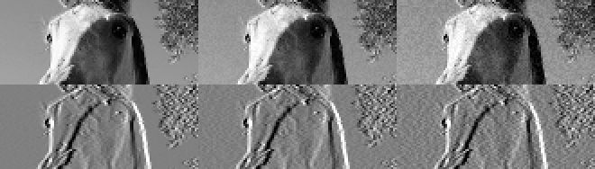
Original

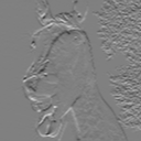
x-direction

$\frac{1}{8}\begin{bmatrix}1 & 0 & -1\\ 2 & 0 & -2\\ 1 & 0& -1 \end{bmatrix}$

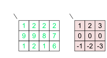
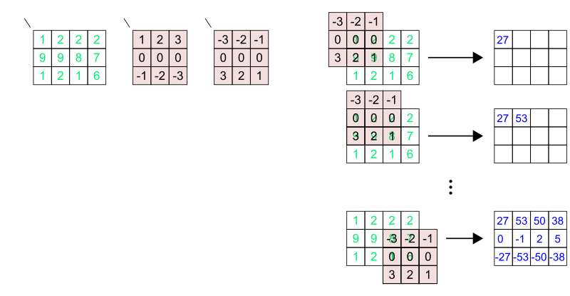
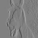
y-direction

$\frac{1}{8}\begin{bmatrix}1 & 2 & 1\\ 0 & 0 & 0\\ -1 & -2& -1 \end{bmatrix}$

Filter Kernels

What is the effect of this filter kernel?
$\begin{bmatrix}0 & -1 & 0\\ -1 & 4 & -1\\ 0 & -1& 0 \end{bmatrix}$

Answer:
- Laplace filter (2nd order derivative)
- Edge filter in $x$-direction and $y$-direction

Separable Filters

For a separable filter kernel, the convolution can be split into several convolutions, i.e.
$\mathrm{f}[x,y] = \mathrm{a}[x,y] \ast \mathrm{b}[x,y] = \left(\mathrm{a}[x,y] \ast \mathrm{b}_1[x,y]\right) \ast \mathrm{b}_2[x,y]$
Here, the separated filter kernels $\mathrm{b}_1[x,y]$ and $\mathrm{b}_2[x,y]$ are smaller and therefore faster to execute
Most of the filter kernels studied so far are x/y-separable, e.g.
$\frac{1}{9}\begin{bmatrix}1 & 1 & 1\\ 1 & 1 & 1\\ 1 & 1& 1 \end{bmatrix} = \frac{1}{3}\begin{bmatrix}1\\ 1\\ 1 \end{bmatrix} \,\, \ast \,\, \frac{1}{3}\begin{bmatrix}1 & 1 & 1\\ \end{bmatrix} $
For a $K \times K$ sized filter kernel, the computational cost is reduced from $K^2$ to $2\, K$ by the separation

Separable Filters

In general, the combined filter kernel of size $K \times K$ results from the x/y-separated kernels of size $K$ by
$ \frac{1}{w_y}\begin{bmatrix}y_1\\ y_2\\ \vdots\\ y_K \end{bmatrix} \,\, \ast \,\, \frac{1}{w_x}\begin{bmatrix}x_1 & x_2 & \dots & x_K\\ \end{bmatrix} = \frac{1}{w_y w_x} \begin{bmatrix}y_1 x_1 & y_1 x_2& \dots & y_1 x_K\\ y_2 x_1 & y_2 x_2& \dots & y_2 x_K \\ \vdots & \vdots & \ddots & \vdots \\ y_K x_1 & y_K x_2&\dots & y_K x_K \end{bmatrix} $
How can this Gaussian filter be separated?
$\frac{1}{16} \begin{bmatrix} 1 & 2 & 1\\ 2 & 4 & 2\\ 1 & 2 & 1 \end{bmatrix}$

Answer:
$\frac{1}{16} \begin{bmatrix} 1 & 2 & 1\\ 2 & 4 & 2\\ 1 & 2 & 1 \end{bmatrix} = \frac{1}{4}\begin{bmatrix}1\\ 2\\ 1 \end{bmatrix} \,\, \ast \,\, \frac{1}{4}\begin{bmatrix}1 & 2 & 1\\ \end{bmatrix} $

Separable Filters

How can this filter, which is responsive to edges in the $x$-direction, be separated?
$\frac{1}{8} \begin{bmatrix}1 & 0 & -1\\ 2 & 0 & -2\\ 1 & 0& -1 \end{bmatrix}$

Answer:
$\frac{1}{8} \begin{bmatrix}1 & 0 & -1\\ 2 & 0 & -2\\ 1 & 0& -1 \end{bmatrix} = \frac{1}{4}\begin{bmatrix}1\\ 2\\ 1 \end{bmatrix} \,\, \ast \,\, \frac{1}{2}\begin{bmatrix}1 & 0 & -1\\ \end{bmatrix} $
Interesting. It is apparently a combination of a Gaussian filter in the $y$-direction and an edge filter in the $x$-direction

Edge Filter

There are two options for edge detection:
- Calculate 1st derivative: The higher the absolute values, the steeper the edge
- Calculate 2nd derivative: Zero crossing at edge

Edge

1st derivative

2nd derivative

Calculate the 1st Derivative

In general, the partial derivatives $\partial \mathrm{f} / \partial x$ and $\partial \mathrm{f} / \partial y$ cannot be determined by the differential quotient for images because the function $\mathrm{f}$ is not an analytic function:
$\frac{\partial \mathrm{f}}{\partial x} = \lim\limits_{x_1 \rightarrow x_0} \frac{\partial \mathrm{f}(x_1) - \mathrm{f}(x_0)}{x_1 - x_0} \quad$ und $\quad \frac{\partial \mathrm{f}}{\partial y} = \lim\limits_{y_1 \rightarrow y_0} \frac{\partial \mathrm{f}(y_1) - \mathrm{f}(y_0)}{y_1 - y_0}$
Instead, the difference quotient is used to approximate the derivative:
$\frac{\mathrm{f}}{\partial x} \approx \frac{\mathrm{f}(x_1) - \mathrm{f}(x_0)}{x_1 - x_0} \quad$ and $\quad \frac{\partial \mathrm{f}}{\partial y} \approx \frac{\partial \mathrm{f}(y_1) - \mathrm{f}(y_0)}{y_1 - y_0}$
For example,
$\frac{\partial \mathrm{f}}{\partial x} \approx \mathrm{f}[x+1,y]- \mathrm{f}[x,y] \quad$ and $\quad \frac{\partial \mathrm{f}}{\partial y} \approx \mathrm{f}[x,y+1]- \mathrm{f}[x,y]$
or also popular, because there is no phase shift:
$\frac{\partial \mathrm{f}}{\partial x} \approx \frac{1}{2} \left( \mathrm{f}[x+1,y]- \mathrm{f}[x-1,y] \right)\quad$ and $\quad \frac{\partial \mathrm{f}}{\partial y} \approx \frac{1}{2} \left( \mathrm{f}[x,y+1] - \mathrm{f}[x,y-1] \right)$

Calculate the 1st Derivative

These calculation
$\frac{\partial \mathrm{f}}{\partial x} \approx \frac{1}{2} \left( \mathrm{f}[x+1,y]- \mathrm{f}[x-1,y] \right)\quad$ and $\quad \frac{\partial \mathrm{f}}{\partial y} \approx \frac{1}{2} \left( \mathrm{f}[x,y+1] - \mathrm{f}[x,y-1] \right)$

can be realized by convolutions with the appropriate filter kernels:

$\frac{\partial \mathrm{f}}{\partial x} \approx \mathrm{f}[x,y] \ast \frac{1}{2}\begin{bmatrix}1 & 0 & -1\end{bmatrix}$

and

$\frac{\partial \mathrm{f}}{\partial y} \approx \mathrm{f}[x,y] \ast \frac{1}{2} \begin{bmatrix}1\\ 0\\ -1 \end{bmatrix}$
This explains why it was chosen as the filter kernel in the example at the beginning

Noise Suppression

Taking the derivative amplifies high frequencies
Image noise typically has a high frequency and is therefore particularly amplified by edge filtering
Therefore, edge filtering can be combined with noise-suppressing low-pass filtering (Gaussian filter) in the orthogonal direction:
$\frac{1}{8} \begin{bmatrix}1 & 0 & -1\\ 2 & 0 & -2\\ 1 & 0& -1 \end{bmatrix} = \frac{1}{4}\begin{bmatrix}1\\ 2\\ 1 \end{bmatrix} \,\, \ast \,\, \frac{1}{2}\begin{bmatrix}1 & 0 & -1\\ \end{bmatrix} $

Sobel Filter

This combination of a low-pass filter and the derivative in x- and y-direction was suggested by Irwin Sobel in 1968 and is therefore called Sobel filter:
$\frac{\partial \mathrm{f}}{\partial x} \approx g_x = \mathrm{f}[x,y] \ast \begin{bmatrix}1 & 0 & -1\\ 2 & 0 & -2\\ 1 & 0& -1 \end{bmatrix} \quad$ and

$\frac{\partial \mathrm{f}}{\partial y} \approx g_y = \mathrm{f}[x,y] \ast \begin{bmatrix}1 & 2 & 1\\ 0 & 0 & 0\\ -1 & -2& -1 \end{bmatrix} $
From the derivatives in x- and y-direction the magnitude of the edge can be computed:
$g = \sqrt{g_x^2 + g_y^2}$
The direction of the edge is given by:
$\theta = \operatorname{atan2}(g_x, g_y)$

Calculate the 2nd Derivative

The second partial derivative can be computed by applying the difference quotient to two neighboring pixels (1st derivative) and then forming the difference quotient on the result (2nd derivative)
For example, for the x-direction:
$\frac{\partial^2 \mathrm{f}}{\partial x^2} \approx \left(\mathrm{f}[x+1,y]- \mathrm{f}[x,y]\right) - \left(\mathrm{f}[x,y]- \mathrm{f}[x-1,y]\right)$

$= \mathrm{f}[x+1,y] - 2 \mathrm{f}[x,y] + \mathrm{f}[x-1,y]$
Expressed as a convolution kernel:
$\frac{\partial^2 \mathrm{f}}{\partial x^2} \approx \mathrm{f}[x,y] \ast \begin{bmatrix}1 & -2 & 1\end{bmatrix}$
Correspondingly in y-direction:
$\frac{\partial^2 \mathrm{f}}{\partial y^2} \approx \mathrm{f}[x,y] \ast \begin{bmatrix}1 \\ -2 \\ 1\end{bmatrix}$

Laplace Operator

Let $\nabla \mathrm{f}$ be a 2-vector containing the 1st derivatives as elements:
$\nabla \mathrm{f}= \begin{pmatrix}\frac{\partial \mathrm{f}}{\partial x} \\\frac{\partial \mathrm{f}}{\partial y}\end{pmatrix} = \underbrace{\begin{pmatrix}\frac{\partial}{\partial x} \\ \frac{\partial}{\partial y}\end{pmatrix} }_{\nabla} \,\,\mathrm{f}$
Then the Laplace operator is defined as the scalar product of $\nabla$ with itself:
$\Delta = \nabla^2 = \nabla^\top \nabla = \begin{pmatrix}\frac{\partial }{\partial x} & \frac{\partial }{\partial y}\end{pmatrix}^\top \begin{pmatrix}\frac{\partial}{\partial x} \\\frac{\partial }{\partial y}\end{pmatrix} = \frac{\partial^2}{\partial x^2} + \frac{\partial^2}{\partial y^2}$
That is, $\Delta \mathrm{f}$ s the sum of the two 2nd derivatives of $\mathrm{f}$:
$\Delta \mathrm{f} = \frac{\partial^2 \mathrm{f}}{\partial x^2} + \frac{\partial^2 \mathrm{f}}{\partial y^2}$

Laplace Filter

In accordance with the Laplace operator, the Laplace filter is defined as the sum of the 2nd derivatives in x- and y-direction
Using the previous result for the filter kernel of the 2nd derivative, we get for the Laplace filter:
$\begin{bmatrix}0 & 1 & 0\\ 1 & -4 & 1\\ 0 & 1& 0 \end{bmatrix} = \begin{bmatrix}0 & 0 & 0\\ 1 & -2 & 1\\ 0 & 0& 0 \end{bmatrix}\,\, + \begin{bmatrix}0 & 1 & 0\\ 0 & -2 & 0\\ 0 & 1& 0 \end{bmatrix} $

Laplacian of Gaussian (LoG)

The Laplace filter amplifies noise particularly strongly due to the 2nd derivative
Therefore, it is usually always combined with a Gaussian filter
Since the order of the convolution does not matter, the input image can also be directly convolved with the combination of a Gauss filter and a Laplace filter
Or the analytical 2nd derivative of a 2D Gaussian function can be used directly:
$\mathrm{b}[x,y] = \exp\left( - \frac{x^2 + \,y^2}{2 \, \sigma^2}\right)$

$\frac{\partial \mathrm{b}}{\partial x} = -\frac{x}{\sigma^2} \exp\left( - \frac{x^2 + \,y^2}{2 \, \sigma^2}\right)$

$\frac{\partial^2 \mathrm{b}}{\partial x^2} = \frac{x^2}{\sigma^4} \exp\left( - \frac{x^2 + \,y^2}{2 \, \sigma^2}\right) - \frac{1}{\sigma^2} \exp\left( - \frac{x^2 + \,y^2}{2 \, \sigma^2}\right) = \frac{x^2-\sigma^2}{\sigma^4} \exp\left( - \frac{x^2 + \,y^2}{2 \, \sigma^2}\right)$

$\Delta \mathrm{b} = \frac{\partial^2 \mathrm{b}}{\partial x^2} + \frac{\partial^2 \mathrm{b}}{\partial y^2} = \frac{x^2 + y^2 - 2\,\sigma^2}{\sigma^4} \exp\left( - \frac{x^2 + \,y^2}{2 \, \sigma^2}\right) $

Laplacian of Gaussian (LoG)

Gauss

$\mathrm{b}[x,y]$

1st derivative

$\frac{\partial \mathrm{b}[x,y]}{\partial x}$

Laplacian of Gaussian

$\Delta \mathrm{b}[x,y]$

Difference of Gaussian

The Difference-of-Gaussian filter is obtained by subtracting the results of two convolutions of Gaussian filters of different strengths
$\mathrm{f}[x,y] = \mathrm{a}[x,y] \ast \frac{1}{\, \sigma_1^2}\exp\left( - \frac{x^2 + \,y^2}{2 \, \sigma_1^2}\right) - \mathrm{a}[x,y] \ast \frac{1}{\, \sigma_2^2} \exp\left( - \frac{x^2 + \,y^2}{2 \, \sigma_2^2}\right)$
whereby $\sigma_1 > \sigma_2$
This gives very similar results to the Laplacian of Gaussian. Why?

Erode

Result

$f[x,y]$

Kernel

Erode is an example of a filter that cannot be implemented with a convolution
Nevertheless, a filter kernel of a certain size is traversed over the image, e.g., 3 x 3, 5 x 5 etc.
The value in the filtered image $\mathrm{f}[x,y]$ is computed by the minimum of all pixels within the filter kernel $\mathcal{K}$ in the input image $\mathrm{a}[x,y]$:
$\mathrm{f}[x,y] = \min\limits_{i,k \,\in\, \mathcal{K}} \left(\mathrm{a}[j,k]\right)$

Dilate

Result

$f[x,y]$

Kernel

For the dilate filter, the maximum is used instead of the minimum
The value in the filtered image $\mathrm{f}[x,y]$ is computed by the maximum of all pixels within the filter kernel $\mathcal{K}$ in the input image $\mathrm{a}[x,y]$:
$\mathrm{f}[x,y] = \max\limits_{i,k \,\in\, \mathcal{K}} \left(\mathrm{a}[j,k]\right)$

Open

Open is used to open structures
First apply Erode, then Dilate

Close

Close is used to connect structures
First apply Dilate, then Erode

Histograms

A histogram contains the number of pixels for each intensity value divided by the total number of pixels
In other words, a histogram describes the relative frequency of intensity values of an image
For example, for an image with 4 x 3 pixels and 5 different intensity values, the result is:

Histograms

The histogram can be calculated on the gray or the color values

Histograms

For example, a histogram can be helpful when taking a picture to check whether the available range of values is well covered.
Overexposed:
Underexposed: