Thorsten Thormählen October 14, 2024 Part 1, Chapter 2
Control Keys
→ move to next slide (also Enter or Spacebar). ← move to previous slide. d enable/disable drawing on slides p toggles between print and presentation view CTRL + zoom in CTRL - zoom out CTRL 0 reset zoom
Slides can also be advanced by clicking on the left or right border of the slide.
Contents
Mechanical Calculating Aids
Mechanical Calculator Machines (from 1600)
Relay-based Computers (from 1941)
Computers based on Electron Tube
Transistor-based Computers (from 1955)
Computers with Integrated Circuits (from 1965)
Microprocessors (from 1971)
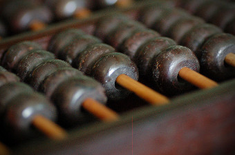
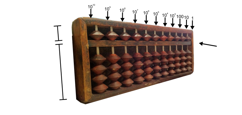
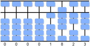
Mechanical Calculating Aids (Abacus), ca. 500 B.C.
Proceed from left to right, one after the other for each digit
Perform addition by simply adding beads
If no matching beads are available, the 5's or 10's complement can be used, for example:
5's complement of 3 is (5 - 3) = 2, i.e. instead of adding 3 beads, add one beads from the heaven and
remove two from the earth
10's complement of 3 is (10 - 3) = 7, add a beads from the next higher digit and remove a total of
seven beads from earth and heaven
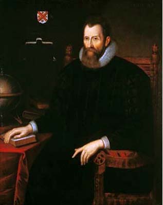
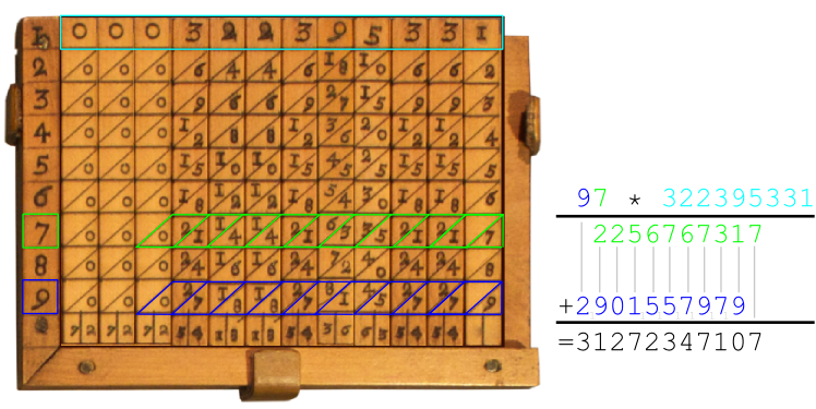
Napier's Bones, 1617
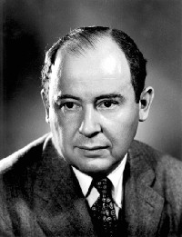
John Napier (1550 - 1617)
In 1617, the Scottish mathematician John Napier described a calculating aid that
can be used to convert a multiplication (or division) into an addition (or subtraction)
For this purpose, the multiplication table is written on rods
The rods are placed on a base board so that the number to be
multiplied is in the top row
The multiplication of the selected number by the factors 2 to 9 can be read in the lines below
The values are read from right to left by adding up the numbers within the resulting parallelograms
An eventual carry-over has to be taken into account
This is an interactive simulator of Napier's bones
Clicking on the individual rods will change their value
Napier's Bones
Example:
Mechanical Calculating Machines (from 1600)
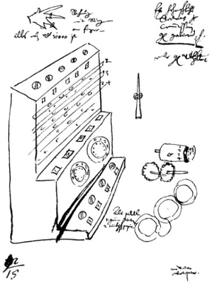
Original drawing of the "calculating clock"
Wilhelm Schickard (1592-1635), a professor in Tübingen, built the first gear-driven calculating machine in
1623
On September 20, 1623, he wrote to Johannes Kepler:
"I recently tried mechanically to do the same thing you did by calculation,
and I built a machine consisting of 11 complete and 6 mutilated wheels,
which automatically adds, subtracts,
multiplies and divides given numbers in an instant.
You would laugh out loud if you were there and could see how,
whenever it goes over a ten or a hundred, the digits on the left
automatically increase or decrease."
The calculating clock by Schickard was capable of automatic addition and subtraction, including automatic
transfer of tens (carry)
The transfer of tens was achieved by means of a toothed wheel construction
Napier's bones (top) were used for multiplication, and the values had to be transferred manually to the
mechanical addition mechanism (bottom)
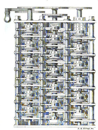
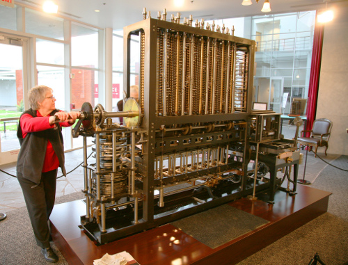
Difference Engine by Charles Babbage, from 1822
Part of the Difference Engine No. 1
"What are you dreaming about? - I am thinking that all these tables of logarithms might be calculated
by machinery."
In 1822, the English mathematics professor Charles Babbage began work on a mechanical calculating machine
for calculating polynomials using Newton's difference method
Unfortunately, he never completed the machine (despite considerable financial support from the British
government until 1842).
The motivation for this was that the written tables used at the time were often inaccurate because they
had been produced manually in monotonous calculations
To avoid copying errors when transferring the results, Babbage had even provided for a printer in a second
version, "Difference Engine No. 2"
In addition to his work on the Difference Engine, Charles Babbage also described a universally applicable
mechanical "Analytic Engine" in 1842
It already had many of the components of today's general-purpose computers (including separation of memory
and arithmetic units, loops, conditional jumps, etc.)
He was way ahead of his time
However, due to the unforeseeable costs, the British government did not want to finance the construction
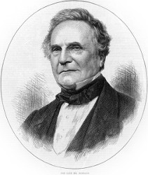
Image source:The Late Mr. Babbage, The Illustrated London News, 4 November 1871, public domain
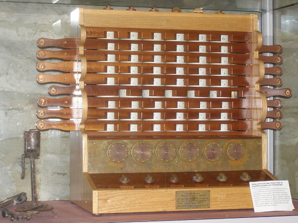
Relay-based Computers
By using electromechanical relays, computers can be designed much more easily than with pure mechanics
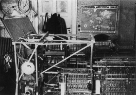
In 1941, the German computer pioneer Konrad Zuse built a fully functional computer out of 2200 relays
Connections for
control voltage
Coil
Movable armature
Contacts
(open)
Contacts
(closed)
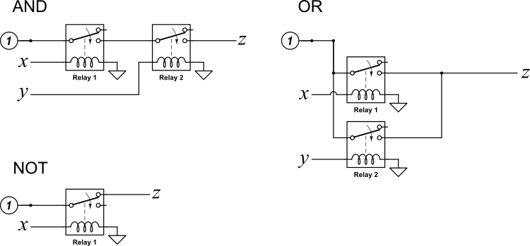
A relay is an electrically controlled on/off switch
No current through coil = armature not magnetically attracted = contact is open
Current through coil = armature is attracted by magnetic field = contact is closed
There are only two states for each switch: on/off (or 1/0)
Based on his experiences with the mechanically operating Z1 (1935 to 1938), Konrad Zuse built a
test model of a relay-based computer in 1939: the Z2
In 1941, he built the Z3, the first relay-based fully functional computer with a clock speed of 5.3 hertz
Relay technology had been used in telecommunications for quite some time at this point
The Z3 had a memory (1600 relays) and a control and arithmetic unit (600 relays).
There were nine commands: input, output, read memory, write memory, multiply, divide, extract root, add,
and subtract.
The commands could be entered directly via a control panel with a keyboard and numeric display
or programmatically using punched tape
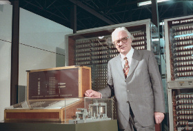
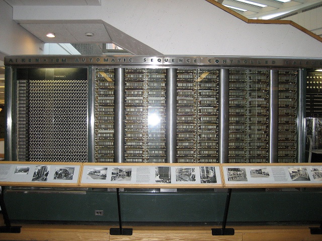
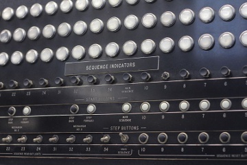
The Harvard Mark I was a relay-based computer designed
by Harvard professor Howard H. Aiken
Aiken began work on the “Automatic Sequence Controlled Calculator” in 1939, which
was completed in 1944 with the support of IBM and was named the "Harvard Mark I"
The commands could be programmatically transferred using punched tape
The calculator was 15.5 meters long and weighed almost 5 tons
IBM had already gained a lot of experience with relay technology and punch cards through its accounting
and tabulating machines
Aiken designed his computer at the same time as Zuse and was not familiar with his work due to the lack of
exchange during the Second World War
In contrast to Zuse, Aiken used decimal arithmetic
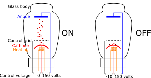
Electron tubes can also be used as switches (triode). They achieve switching times that are 1000 to 2000
times faster than the best relays.
In a vacuum, electrons are emitted from the heated cathode and are attracted by the strong positive charge
of the anode
No voltage at the control grid = current flows
Negative voltage at the control grid = no current flows
This means that there are two states again (just like with a relay): on/off (or 1/0)
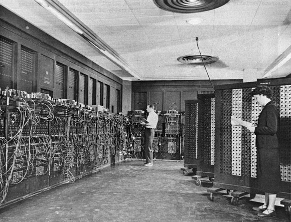
ENIAC, the first entirely electronic computer, 1946
"Electronic Numerical Integrator and Computer" (ENIAC)
Image source:Eniac,
U.S. Army Photo, public domain
ENIAC, 1946
ENIAC was developed from 1942 by John W. Mauchly and Persper Eckert at the Moore School of Electrical
Engineering, University of Pennsylvania, and presented to the public in 1946
It took up an entire room, weighed about 30 tonnes and consisted of 17,468 electron tubes, 7,200 diodes,
1,500 relays, 70,000 resistors and 10,000 capacitors
Thanks to the electron tubes, the ENIAC was faster (approx. 1000 Hz) than relay-based computers, but it had
the following disadvantages:
Very high power consumption (174,000 watts)
The tubes break quickly (average service life of about two years, which meant that on average, a
tube was broken every hour). The modular design made it possible to replace entire modules.
Programming was done by rewiring the device, which meant that the ENIAC was not very flexible. Its main
task was to calculate ballistic tables for the U.S. Army
Image source:Eniac, U.S.
Army Photos, public domain
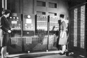
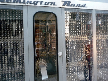
UNIVAC I, 1951
Eckert and Mauchly founded the "Eckert-Mauchly Computer Corporation" to commercialise their invention
The successor to the ENIAC was the UNIVAC I (UNIVersal Automatic Computer)
The UNIVAC was memory-programmable and could store data on magnetic tape (12,800 characters per second)
After being taken over by Remington Rand, 46 systems were sold
UNIVAC I computer in the "Deutsches Museum", Munich
At the Institute for Advanced Study (IAS) in Princeton, John von Neumann developed a computer based on
electronic tubes that,
unlike ENIAC, worked in binary code
As early as 1944, von Neumann and Eckert and Mauchly had described a concept for a universal computer
(initially only in theory)
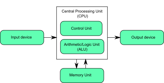
The von Neumann computer architecture concept states:
The structure of the computer is independent of the problem to be solved
There are five functional units: control unit, arithmetic/logic unit, memory unit, input and output device
Von Neumann Computer Architecture
Commands and data are binary-coded and stored in a joint memory
The memory is divided into equally-sized cells that can be addressed with consecutive numbers
Instructions that are stored in succession in the memory are executed in succession
Jump commands can change the order of execution
The memory (data and instructions) can be modified by the machine
The concept is still popular because the programming is quite simple due to the strictly sequential
process (nothing happens in parallel).
Transistor-based Computers
Electron tubes were unreliable and have been replaced by a new electronic component since the early 1950s:
the transistor
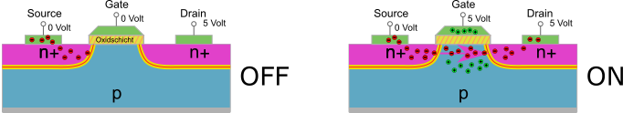
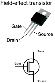
The field-effect transistor shown here consists of p- and n-doped semiconductor material. There are three
metal contacts: source, drain and gate
The current between source and drain is controlled by the voltage between gate and source.
0 volts at the gate = the electrons cannot overcome the p-doped region = no current flows
5 volts at the gate = electrons accumulate below the gate (n-channel) = electrons flow through channel =
current flows
This means that there are two states again: on/off (or 1/0)
TRADIC, 1955
TRADIC (TRansistorised Airborne DIgital Computer) was developed by AT&T Bell Labs for the US Air Force and
went into operation in 1955
Instead of electron tubes, around 700-800 individual transistors were used
In addition to the probability of failure and the reduces size, the power consumption was also reduced to
approx. 100 watts.
The computing speed was already around one million logical operations per second (1 MHz)
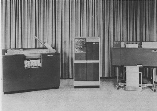
IBM 1401, 1959
IBM 1401 was a large computer designed for processing mass data (census, accounting, customer data, etc.)
in
large companies or government institutions
A total of more than 10,000 units were built
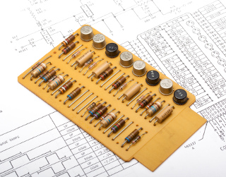
The logic circuits were built from individual PCBs with wired components (transistors, capacitors, and
diodes).
The basic configuration had a punched card reader (on the left in the figure) and a printer (right).
Several magnetic tape units could be connected (transfer speed 41,000 characters per second).
The IBM 1401 could be programmed with the high-level programming language FORTRAN, among others
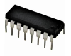
Instead of manufacturing individual transistors as discrete components, many transistors are
integrated on a single piece of semiconductor material (integrated circuit, IC)
In 1958, Jack Kibly of Texas Instruments succeeded in producing the first integrated circuit
A few years later, the ICs were ready for the market. The first computer system to
use them commercially was the IBM /360 computers.
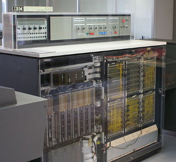
IBM /360, 1965
Introduction of a family concept: all computers in a family are compatible
Idea: All machines have the same machine instruction set. The implementation on different physical
hardware is done by microprogramming
A microprogram specifies how the individual logic modules are to be controlled when executing a particular
machine command (e.g. addition)
IBM /360 Model 85 was the first commercial system to use a cache (fast local memory that stores a copy of
the main memory data)
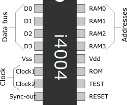
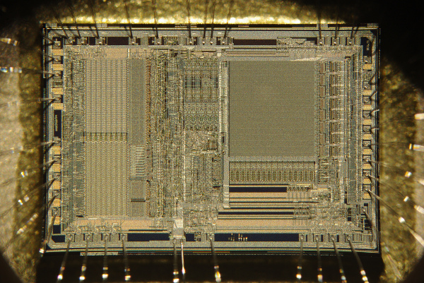
Intel 4004: the first microprocessor by Intel, 1971
Intel (Integrated Electronics Corporation) was founded in 1968 by Gordon Moore and Robert Noyce
In November 1971, Intel's first microprocessor, the 4004, came into the market
The IC was manufactured with a process size of 10 micrometres. It had 2250 transistors and initially
operated at a clock rate of 108 KHz
The 4004 has a 4-bit data bus, i.e. only 4 on/off states (= 4 bits) can be read per bus clock
However, one command was coded as a sequence of 8 ones/zeros, e.g. 01101000. Therefore,
the data bus worked twice as fast in order to be able to read one command per processor cycle
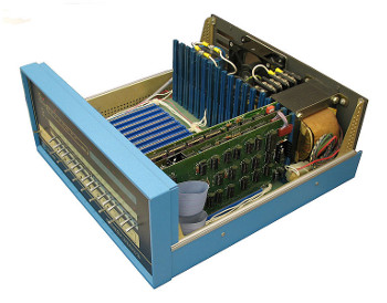
Intel 8080, 1974
Altair 8800 with Intel 8080 CPU
In April 1974, Intel introduced the 8080, which many consider to be the first truly usable microprocessor
The Intel 8080 and its predecessor, the 8008 (1972), were 8-bit computers, i.e. 8 bits (= 1 byte) could be
processed within one clock cycle
The 8080 has an 8-bit data bus and a 16-bit address bus. This made it possible to address (2 to the power
of 16) = 65536 bytes in the external memory
The IC was manufactured with a process size of 6 micrometres. It had 4,500 transistors and operated at a
clock speed of 2 MHz
From 1975, hobbyists were able to order the low-cost Altair 8800 home-assembly computer kit, based on the
8080
This marked the arrival of the computer in the homes of technology enthusiasts:
The personal computer (PC) was born
The Apple II was comparatively low-priced and was the first personal computer to become widespread. The
first
big commercial success for the founders of Apple: Steve Wozniak and Steve Jobs
Interestingly, the Apple II's blueprints were made public, meaning that other manufacturers could expand
on it – but also replicate it
In addition to text, the Apple II was already capable of displaying color graphics: either 15 colors at
low resolution (40 × 48 pixels) or 6 colors at high resolution (280 × 192 pixels)
The Intel 8086 was manufactured with a process size of 3 micrometers, had 29,000 transistors and operated
at a clock speed of 5 to 10 MHz
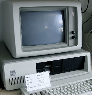
The x86 microprocessor architecture, named after the 8086, would later become an industry standard, mainly
because IBM started using a later version of the processor, the Intel 8088, in their PCs in 1981
The IBM PC was a huge success. It was also copied many times, with compatible PCs built with the same
components
Consequently, the x86 microprocessor architecture has seen widespread use
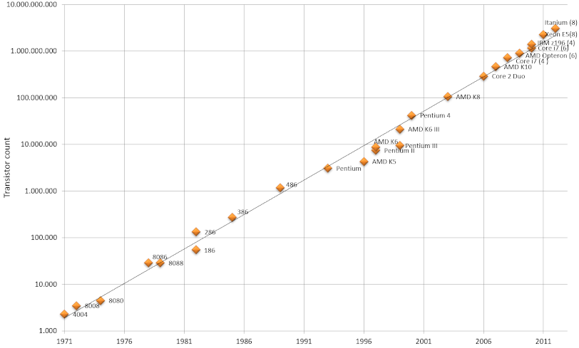
"The complexity for minimum component costs has increased at a rate of roughly a factor of two per year.
Certainly over the short term this rate can be expected to continue, if not to increase. Over the longer
term, the rate of increase is a bit more uncertain, although
there is no reason to believe it will not remain nearly constant for at least ten years" - Gordon E. Moore,
1965
In 1975, Moore changed his statement and predicted that the number of transistors on a microchip would
double every two years (sometimes the literature also speaks of a doubling every 18 months).
The exact time span is not important in this statement. What is important is that the number of
transistors is growing exponentially
Microchip manufacturers are trying to maintain this exponential growth (a self-fulfilling prophecy),
although
it has often been predicted that Moore's Law would end due to technological limitations
Since 2006, clock rates have no longer increased significantly, but several processing units (cores) have
been placed on one chip
Source: Gordon E. Moore, “Cramming More Components onto Integrated Circuits,” Electronics, pp. 114–117,
April 19, 1965.
As the machine instructions of the established architectures became more and more involved and complex, a
countermovement arose in the 1980s
Computers with the traditional instruction sets were referred to as:
CISC (Complex Instruction Set Computer)
A new computer architecture was proposed:
RISC (Reduced Instruction Set Computer)
The simple RISC instructions are faster to execute and take roughly the same time each
The simple instructions use dedicated hardware and replace the microprogramming that is common in CISC
processors
The RISC processors can therefore be run at a faster clock speed and the pipelining of instruction
sequences
becomes more efficient
Motorola 68000, PowerPC (Apple), ARM (Smartphone) are further examples of RISC processors
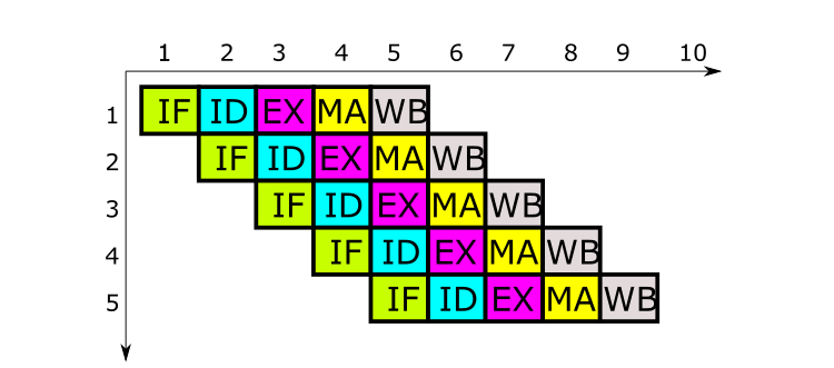
Pipelining
Multiple tasks are processed simultaneously with multiple resources
In the MIPS architecture, for example, dedicated hardware for: Instruction Fetch (IF), Instruction Decode
(ID), Execute (EX), Memory Accesss (MA), and
Write Back (WB)
Therefore, pipelining can achieve up to five times the speed of sequential execution
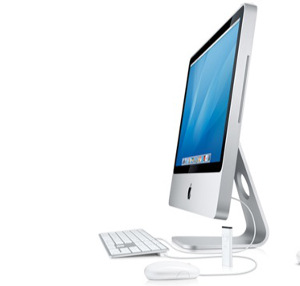
Especially since the iMac, Apple has placed a lot of emphasis on design
Apple's idea: the iMac integrates the monitor and computer hardware into a single housing, which is not
usual.
This prevents cable clutter on the desk, but has the disadvantage that components cannot be easily replaced.
The concept is still in use today (top: iMac G3 from 1998; bottom: iMac from 2007)
The iMac G3 had a 233 MHz PowerPC CPU with 512 KB cache, 4 GB hard disk, 32 MB RAM, 2 MB video RAM and
came with Mac OS 8.1