Graphics Programming
Image-based Lighting
Thorsten Thormählen
January 09, 2022
Part 10, Chapter 2
Thorsten Thormählen
January 09, 2022
Part 10, Chapter 2
This is the print version of the slides.
Advance slides with the → key or
by clicking on the right border of the slide
Slides can also be advanced by clicking on the left or right border of the slide.
| Type | Font | Examples |
|---|---|---|
| Variables (scalars) | italics | $a, b, x, y$ |
| Functions | upright | $\mathrm{f}, \mathrm{g}(x), \mathrm{max}(x)$ |
| Vectors | bold, elements row-wise | $\mathbf{a}, \mathbf{b}= \begin{pmatrix}x\\y\end{pmatrix} = (x, y)^\top,$ $\mathbf{B}=(x, y, z)^\top$ |
| Matrices | Typewriter | $\mathtt{A}, \mathtt{B}= \begin{bmatrix}a & b\\c & d\end{bmatrix}$ |
| Sets | calligraphic | $\mathcal{A}, B=\{a, b\}, b \in \mathcal{B}$ |
| Number systems, Coordinate spaces | double-struck | $\mathbb{N}, \mathbb{Z}, \mathbb{R}^2, \mathbb{R}^3$ |
| Symbol | Meaning |
|---|---|
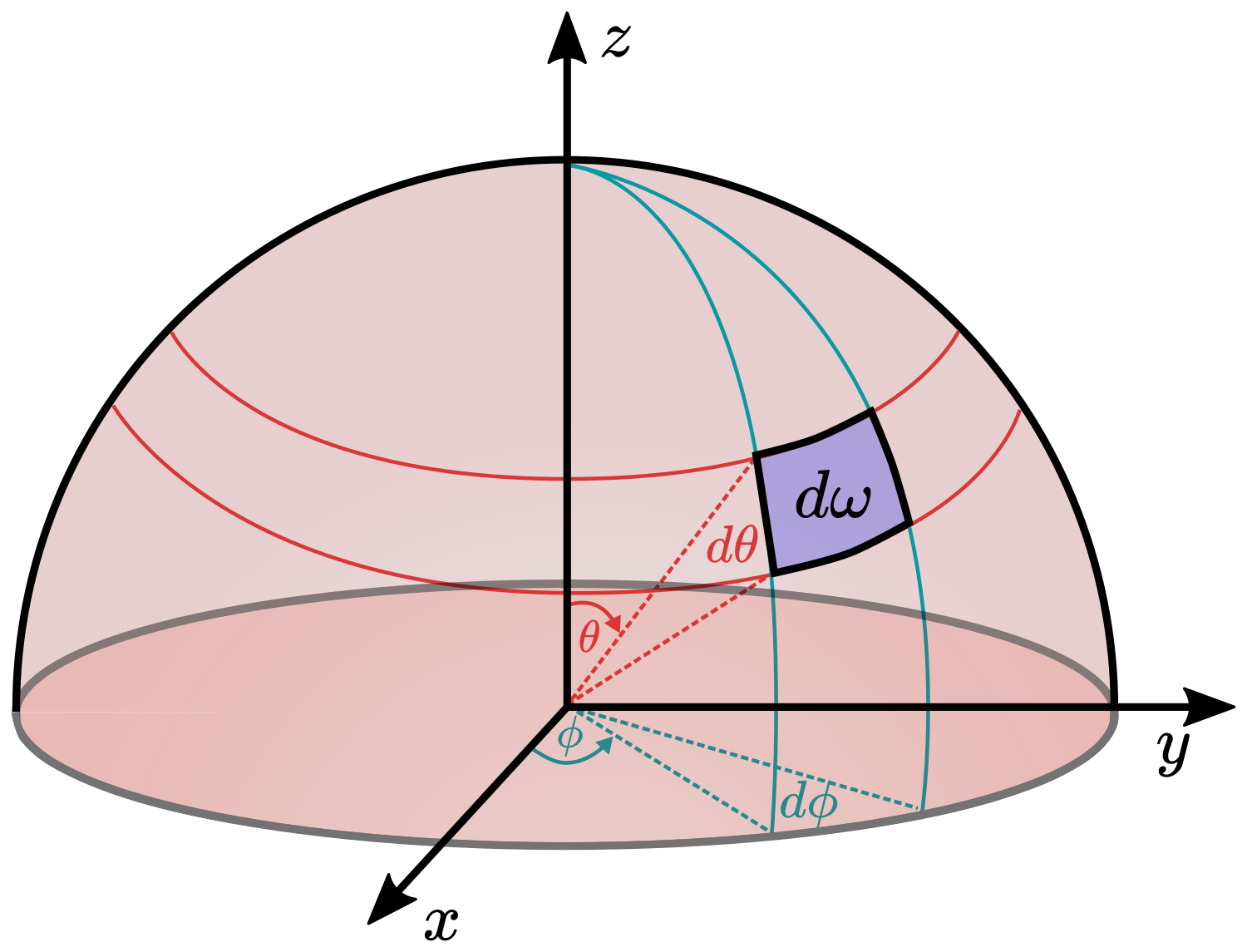
| $\Omega$ | Solid angle |
| $\theta$ | Polar angle in the spherical coordinate system |
| $\phi$ | Azimuth angle in the spherical coordinate system |
| $\Phi$ | Radiant flux |
| $I$ | Radiant intensity |
| $E$ | Irradiance |
| $L$ | Radiance |
| $\mathrm{f}_r$ | BRDF (Bidirectional Reflection Distribution Function) |
| $\mathrm{f}_d$ | Diffuse part of the BRDF |
| $\mathrm{f}_s$ | Specular part of the BRDF |
| Symbol | Meaning |
|---|---|
| $\mathbf{n}$ | Surface normal |
| $\mathbf{v}$ | Unit vector in view direction |
| $\mathbf{l}$ | Unit vector in light direction |
| $\eta$ | Refractive index |
| $F$ | Fresnel reflectance |
| $\mathbf{h}$ | Halfway vector between light and view direction |
| $(\dots)_+$ | Ramp function |
| $\langle \mathbf{a}\cdot \mathbf{b}\rangle$ | Scalar product |
| PDF / Mapping | Top view | Side view |
|---|---|---|
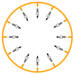
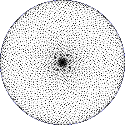
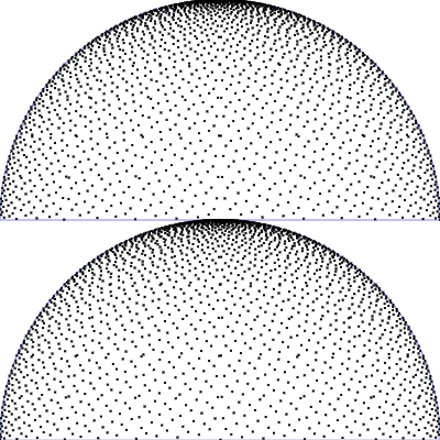
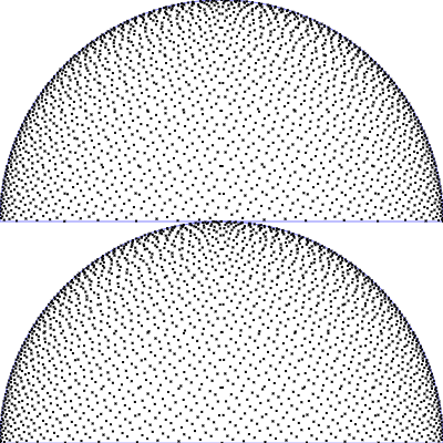
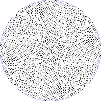
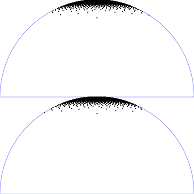
| Uniform sampling of polar angles
$\mathrm{p}(\theta, \phi) = \frac{1}{2\pi} \frac{1}{\pi/2}$
$\phi = 2 \pi \,u$
$\theta = \frac{\pi}{2}\, v$
(corresponds to the Riemann sum)
|
|
|
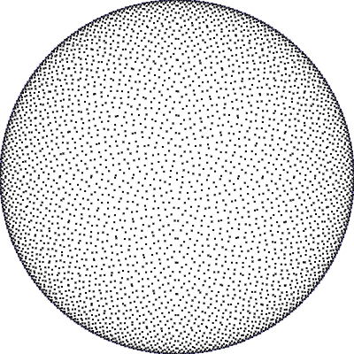
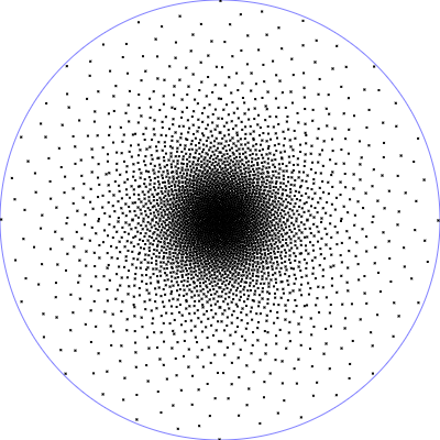
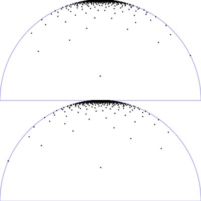
| Uniform sampling of a hemisphere
$\mathrm{p}(\theta, \phi) = \frac{1}{2\pi} \,\sin(\theta)$
$\phi = 2 \pi \,u$
$\theta = \arccos(1 - v)$
|
|
|
| PDF / Mapping | Top view | Side view |
|---|---|---|
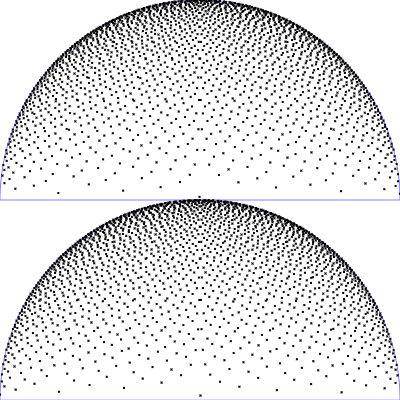
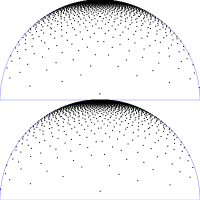
| Phong BRDF (diffuse part)
$\mathrm{p}(\theta, \phi) = \frac{1}{\pi} \, \cos(\theta) \,\sin(\theta)$
$\phi = 2 \pi \,u$
$\theta = \arcsin(\sqrt{v})$
|
|
|
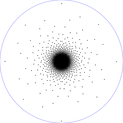
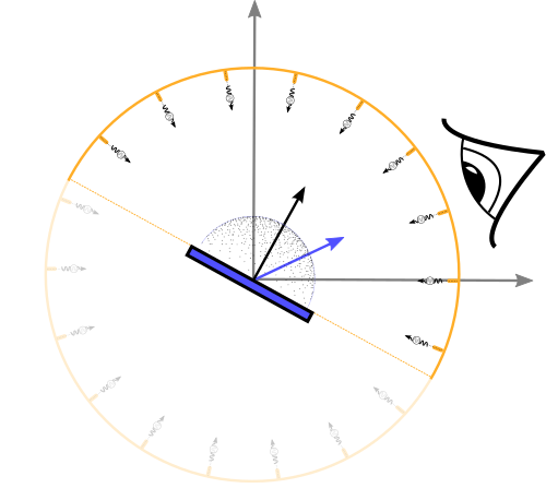
| Phong BRDF (specualar part)
$\mathrm{p}(\theta, \phi) = \frac{n_s + 1}{2 \pi} \, \cos(\theta)^{n_s} \,\sin(\theta)$
$\phi = 2 \pi \,u$
$\theta = \arccos\left((1-v)^{\frac{1}{n_s+1}}\right)$
|
|
|
| PDF / Mapping | Top view | Side view |
|---|---|---|
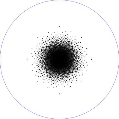
| Microfacet GGX distribution with $r_p = 0.5$ und $\alpha = r_p^2$
$\mathrm{D}_{\tiny \mbox{GGX}}(\theta) = \frac{\alpha^2}{\pi \left(\cos^2(\theta) (\alpha^2-1)+1\right)^2}$
$\mathrm{p}(\theta, \phi) = \mathrm{D}_{\tiny \mbox{GGX}}(\theta)\cos(\theta)\sin(\theta)$
$\phi = 2 \pi \,u$
$\theta = \arccos\left(\sqrt{\frac{1 - v}{v (\alpha^2-1) + 1} }\right)$
|
|
|
| Microfacet GGX distribution with $r_p = 0.25$ |
|
|

| Index $n$ | Numerical value (Base 2) | Mirrored | $h_2(n)$ |
|---|---|---|---|
| 1 | 1 | 0.1 = 1/2 | 0.5 |
| 2 | 10 | 0.01 = 1/4 | 0.25 |
| 3 | 11 | 0.11 = 3/4 | 0.75 |
| 4 | 100 | 0.001 = 1/8 | 0.125 |
| 5 | 101 | 0.101 = 1/2 + 1/8 | 0.625 |
| 6 | 110 | 0.011 = 1/4 + 1/8 | 0.375 |
| 7 | 111 | 0.111 = 1/2 + 1/4 + 1/8 | 0.875 |

| Index $n$ | Numerical value (Base 3) | Mirrored | $h_3(n)$ |
|---|---|---|---|
| 1 | 1 | 0.1 = 1/3 | 0.333 |
| 2 | 2 | 0.2 = 2/3 | 0.666 |
| 3 | 10 | 0.01 = 1/9 | 0.111 |
| 4 | 11 | 0.11 = 1/3 + 1/9 | 0.444 |
| 5 | 12 | 0.21 = 2/3 + 1/9 | 0.777 |
| 6 | 20 | 0.02 = 2/9 | 0.222 |
| 7 | 21 | 0.12 = 1/3 + 2/9 | 0.555 |
| 8 | 22 | 0.22 = 2/3 + 2/9 | 0.888 |


Important sampling of the diffuse part:
#version 300 es
precision highp float;
out vec4 outColor;
in vec2 tc; // texture coordinate of the output image in range [0.0, 1.0]
uniform int samples; // number of samples
uniform float envMapLevel; // environment map level
uniform sampler2D envMapImage; // environment image

const float PI = 3.1415926535897932384626433832795;

vec2 directionToSphericalEnvmap(vec3 dir) {
  float s = 1.0 - mod(1.0 / (2.0*PI) * atan(dir.y, dir.x), 1.0);
  float t = 1.0 / (PI) * acos(-dir.z);
  return vec2(s, t);
}

mat3 getNormalSpace(in vec3 normal) {
   vec3 someVec = vec3(1.0, 0.0, 0.0);
   float dd = dot(someVec, normal);
   vec3 tangent = vec3(0.0, 1.0, 0.0);
   if(abs(dd) > 1e-8) {
     tangent = normalize(cross(someVec, normal));
   }
   vec3 bitangent = cross(normal, tangent);
   return mat3(tangent, bitangent, normal);
}

// from http://holger.dammertz.org/stuff/notes_HammersleyOnHemisphere.html
// Hacker's Delight, Henry S. Warren, 2001
float radicalInverse(uint bits) {
  bits = (bits << 16u) | (bits >> 16u);
  bits = ((bits & 0x55555555u) << 1u) | ((bits & 0xAAAAAAAAu) >> 1u);
  bits = ((bits & 0x33333333u) << 2u) | ((bits & 0xCCCCCCCCu) >> 2u);
  bits = ((bits & 0x0F0F0F0Fu) << 4u) | ((bits & 0xF0F0F0F0u) >> 4u);
  bits = ((bits & 0x00FF00FFu) << 8u) | ((bits & 0xFF00FF00u) >> 8u);
  return float(bits) * 2.3283064365386963e-10; // / 0x100000000
}

vec2 hammersley(uint n, uint N) {
  return vec2(float(n) / float(N), radicalInverse(n));
}

void main() {

  float thetaN = PI * (1.0 - tc.y);
  float phiN = 2.0 * PI * (1.0 - tc.x);
  vec3 normal = vec3(sin(thetaN) * cos(phiN),
                     sin(thetaN) * sin(phiN),
                     cos(thetaN));
  mat3 normalSpace = getNormalSpace(normal);

  vec3 result = vec3(0.0);

  uint N = uint(samples);

  float r = random2(tc);

  for(uint n = 1u; n <= N; n++) {
      vec2 p = hammersley(n, N);
      float theta = asin(sqrt(p.y));
      float phi = 2.0 * PI * p.x;
      vec3 pos = vec3(sin(theta) * cos(phi), sin(theta) * sin(phi), cos(theta));
      vec3 posGlob = normalSpace * pos;
      vec2 uv = directionToSphericalEnvmap(posGlob);
      vec3 radiance = textureLod(envMapImage, uv, envMapLevel).rgb;
      result +=  radiance;
  }
  result = result / float(samples);
  outColor.rgb = result;
  outColor.a = 1.0;
}Important sampling of the specular part:
#version 300 es
precision highp float;
out vec4 outColor;
in vec2 tc; // texture coordinate of the output image in range [0.0, 1.0]
uniform int samples; // number of samples
uniform float shininess; // specular shininess exponent
uniform float envMapLevel; // environment map level
uniform sampler2D envMapImage; // environment image
const float PI = 3.1415926535897932384626433832795;

vec2 directionToSphericalEnvmap(vec3 dir) {
  float s = 1.0 - mod(1.0 / (2.0*PI) * atan(dir.y, dir.x), 1.0);
  float t = 1.0 / (PI) * acos(-dir.z);
  return vec2(s, t);
}

mat3 getNormalSpace(in vec3 normal) {
   vec3 someVec = vec3(1.0, 0.0, 0.0);
   float dd = dot(someVec, normal);
   vec3 tangent = vec3(0.0, 1.0, 0.0);
   if(abs(dd) > 1e-8) {
     tangent = normalize(cross(someVec, normal));
   }
   vec3 bitangent = cross(normal, tangent);
   return mat3(tangent, bitangent, normal);
}

// from http://holger.dammertz.org/stuff/notes_HammersleyOnHemisphere.html
// Hacker's Delight, Henry S. Warren, 2001
float radicalInverse(uint bits) {
  bits = (bits << 16u) | (bits >> 16u);
  bits = ((bits & 0x55555555u) << 1u) | ((bits & 0xAAAAAAAAu) >> 1u);
  bits = ((bits & 0x33333333u) << 2u) | ((bits & 0xCCCCCCCCu) >> 2u);
  bits = ((bits & 0x0F0F0F0Fu) << 4u) | ((bits & 0xF0F0F0F0u) >> 4u);
  bits = ((bits & 0x00FF00FFu) << 8u) | ((bits & 0xFF00FF00u) >> 8u);
  return float(bits) * 2.3283064365386963e-10; // / 0x100000000
}

vec2 hammersley(uint n, uint N) {
  return vec2(float(n) / float(N), radicalInverse(n));
}

void main() {

  float thetaN = PI * (1.0 - tc.y);
  float phiN = 2.0 * PI * (1.0 - tc.x);
  vec3 normal = vec3(sin(thetaN) * cos(phiN),
                     sin(thetaN) * sin(phiN),
                     cos(thetaN));
  mat3 normalSpace = getNormalSpace(normal);

  vec3 result = vec3(0.0);

  uint N = uint(samples);

  float r = random2(tc);

  for(uint n = 1u; n <= N; n++) {
      vec2 p = hammersley(n, N);
      float theta = acos(pow(1.0 - p.y, 1.0/(shininess + 1.0)));
      float phi = 2.0 * PI * p.x;
      vec3 pos = vec3(sin(theta) * cos(phi), sin(theta) * sin(phi), cos(theta));
      vec3 posGlob = normalSpace * pos;
      vec2 uv = directionToSphericalEnvmap(posGlob);
      vec3 radiance = textureLod(envMapImage, uv, envMapLevel).rgb;
      result +=  radiance;
  }
  result = result / float(samples) * (shininess + 2.0) / (shininess + 1.0);
  outColor.rgb = result;
  outColor.a = 1.0;
}Vertex shader for the result image:
#version 300 es
precision highp float;
in vec3 position; // input vertex position from mesh
in vec2 texcoord; // input vertex texture coordinate from mesh
in vec3 normal;   // input vertex normal from mesh

uniform mat4 cameraLookAt; //camera look at matrix
uniform mat4 cameraProjection; //camera projection matrix
uniform mat4 meshTransform0; // mesh0 transformation
uniform mat4 meshTransform1; // mesh1 transformation
uniform mat4 meshTransform0TransposedInverse;
uniform mat4 meshTransform1TransposedInverse;

uniform int gsnMeshGroup;

out vec2 tc; // output texture coordinate of vertex
out vec3 wfn; // output fragment normal of vertex in world space
out vec3 vertPos; // output 3D position in world space

void main(){
  mat4 meshTransform;
  mat4 meshTransformTransposedInverse;

  if(gsnMeshGroup == 0) {  // transformation of background sphere
   meshTransform = meshTransform0;
   meshTransformTransposedInverse = meshTransform0TransposedInverse;
  } else { // transformation of mesh
   meshTransform = meshTransform1;
   meshTransformTransposedInverse = meshTransform1TransposedInverse;
  }
  tc = texcoord;
  wfn = vec3(meshTransformTransposedInverse * vec4(normal, 0.0));
  vec4 vertPos4 = meshTransform * vec4(position, 1.0);
  vertPos = vec3(vertPos4) / vertPos4.w;
  gl_Position = cameraProjection * cameraLookAt * vertPos4;
}Fragment shader for the result image:
#version 300 es
precision highp float;
precision highp int;
out vec4 outColor;

#define M_PI 3.1415926535897932384626433832795

in vec2 tc; // texture coordinate of pixel (interpolated)
in vec3 wfn; // fragment normal of pixel in world space (interpolated)
in vec3 vertPos; // fragment vertex position in world space (interpolated)

uniform sampler2D envmapBackground; // min_filter="LINEAR" mag_filter="LINEAR"
uniform bool showBackground; // defaultval="true"
uniform sampler2D envmapDiffuse; // min_filter="LINEAR" mag_filter="LINEAR"
uniform sampler2D envmapSpecular; // min_filter="LINEAR" mag_filter="LINEAR"
uniform float diffuseMix; // weighting factor of diffuse color
uniform vec4 diffuseColor; // diffuse color
uniform float specularMix; // weighting factor of specular color
uniform vec4 specularColor; // pecularColor
uniform vec3 cameraPos; // camera position in global coordinate system
uniform int gsnMeshGroup;

vec2 directionToSphericalEnvmap(vec3 dir) {
  float s = 1.0 - mod(1.0 / (2.0*M_PI) * atan(dir.y, dir.x), 1.0);
  float t = 1.0 / (M_PI) * acos(-dir.z);
  return vec2(s, t);
}

void main() {
  vec3 normal = normalize(wfn.xyz);
  vec3 viewDir = normalize(cameraPos - vertPos);

  vec3 rv = reflect(-viewDir, normal);

  if(gsnMeshGroup == 0) {
    if(showBackground) {
      // color of envmap sphere
      outColor.rgb = texture(envmapBackground, vec2(1.0-tc.x, tc.y)).rgb;
      outColor.a = 1.0;
    } else {
      discard;
    }
  } else {

    vec3 diff = texture(envmapDiffuse, directionToSphericalEnvmap(normal)).rgb;
    vec3 rd = diffuseMix * pow(diffuseColor.rgb, vec3(2.2));
    vec3 rs = specularMix * pow(specularColor.rgb, vec3(2.2));

    // shading front-facing
    vec3 color = rd * diff;
    float rn = dot(rv, normal);
    if(rn > 0.0) {
      vec3 spec = texture(envmapSpecular, directionToSphericalEnvmap(rv)).rgb;
      color += rs * rn * spec;
    }

    // shading back-facing
    if(dot(viewDir, normal) < -0.1) {
      color = 0.1 * rs;
    }

    outColor.rgb = pow(color, vec3(1.0/2.2));
    outColor.a = 1.0;
  }
}
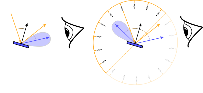
with $\theta^\ast = 2 \,\theta_h^\ast$ and $\phi^\ast = \phi_h^\ast$
Fragment shader (vertex shader as before):
#version 300 es
precision highp float;
precision highp int;
out vec4 outColor;

#define PI 3.1415926535897932384626433832795

in vec2 tc; // texture coordinate of pixel (interpolated)
in vec3 wfn; // fragment normal of pixel (interpolated)
in vec3 vertPos; // fragment vertex position (interpolated)

uniform sampler2D envMapImage; // environment images
uniform sampler2D baseColorTexture; // base color
uniform sampler2D roughnessTexture; // roughness texture
uniform sampler2D metallicTexture; // metallic parameter
uniform sampler2D emissionTexture; // emission texture
uniform float reflectance; // Fresnel reflectance
uniform bool showBackground;
uniform int samplesSpec; //number of samples
uniform float envLevelSpec; // level for envmap lookup
uniform int samplesDiff; // number of samples
uniform float envLevelDiff; // level for envmap lookup
uniform vec3 cameraPos; // camera position in global coordinate system
uniform int gsnMeshGroup;

vec2 directionToSphericalEnvmap(vec3 dir) {
  float s = 1.0 - mod(1.0 / (2.0*PI) * atan(dir.y, dir.x), 1.0);
  float t = 1.0 / (PI) * acos(-dir.z);
  return vec2(s, t);
}

mat3 getNormalSpace(in vec3 normal) {
   vec3 someVec = vec3(1.0, 0.0, 0.0);
   float dd = dot(someVec, normal);
   vec3 tangent = vec3(0.0, 1.0, 0.0);
   if(abs(dd) > 1e-8) {
     tangent = normalize(cross(someVec, normal));
   }
   vec3 bitangent = cross(normal, tangent);
   return mat3(tangent, bitangent, normal);
}

// from http://holger.dammertz.org/stuff/notes_HammersleyOnHemisphere.html
// Hacker's Delight, Henry S. Warren, 2001
float radicalInverse(uint bits) {
  bits = (bits << 16u) | (bits >> 16u);
  bits = ((bits & 0x55555555u) << 1u) | ((bits & 0xAAAAAAAAu) >> 1u);
  bits = ((bits & 0x33333333u) << 2u) | ((bits & 0xCCCCCCCCu) >> 2u);
  bits = ((bits & 0x0F0F0F0Fu) << 4u) | ((bits & 0xF0F0F0F0u) >> 4u);
  bits = ((bits & 0x00FF00FFu) << 8u) | ((bits & 0xFF00FF00u) >> 8u);
  return float(bits) * 2.3283064365386963e-10; // / 0x100000000
}

vec2 hammersley(uint n, uint N) {
  return vec2(float(n) / float(N), radicalInverse(n));
}

float random2(vec2 n) {
	return fract(sin(dot(n, vec2(12.9898, 4.1414))) * 43758.5453);
}

float G1_GGX_Schlick(float NdotV, float roughness) {
  float r = roughness; // original
  //float r = 0.5 + 0.5 * roughness; // Disney remapping
  float k = (r * r) / 2.0;
  float denom = NdotV * (1.0 - k) + k;
  return NdotV / denom;
}

float G_Smith(float NoV, float NoL, float roughness) {
  float g1_l = G1_GGX_Schlick(NoL, roughness);
  float g1_v = G1_GGX_Schlick(NoV, roughness);
  return g1_l * g1_v;
}

vec3 fresnelSchlick(float cosTheta, vec3 F0) {
  return F0 + (1.0 - F0) * pow(1.0 - cosTheta, 5.0);
}

// adapted from "Real Shading in Unreal Engine 4", Brian Karis, Epic Games
vec3 specularIBLReference(vec3 F0 , float roughness, vec3 N, vec3 V) {
  mat3 normalSpace = getNormalSpace(N);
  vec3 result = vec3(0.0);
  uint sampleCount = uint(samplesSpec);
  float r = random2(tc);
  for(uint n = 1u; n <= sampleCount; n++) {
    //vec2 p = hammersley(n, N);
    vec2 p = mod(hammersley(n, sampleCount) + r, 1.0);
    float a = roughness * roughness;
    float theta = acos(sqrt((1.0 - p.y) / (1.0 + (a * a - 1.0) * p.y)));
    float phi = 2.0 * PI * p.x;
    // sampled h direction in normal space
    vec3 Hn = vec3(sin(theta) * cos(phi), sin(theta) * sin(phi), cos(theta));
    // sampled h direction in world space
    vec3 H = normalSpace * Hn;
    vec3 L = 2.0 * dot(V, H) * H - V;

    // all required dot products
    float NoV = clamp(dot(N, V), 0.0, 1.0);
    float NoL = clamp(dot(N, L), 0.0, 1.0);
    float NoH = clamp(dot(N, H), 0.0, 1.0);
    float VoH = clamp(dot(V, H), 0.0, 1.0);
    if(NoL > 0.0 && NoH > 0.0 && NoV > 0.0 && VoH > 0.0) {
      // geometry term
      float G = G_Smith(NoV, NoL, roughness);

      // Fresnel term
      vec3 F = fresnelSchlick(VoH, F0);

      vec2 uv = directionToSphericalEnvmap(L);
      vec3 radiance = textureLod(envMapImage, uv, envLevelSpec).rgb;
      result += radiance * F * G * VoH / (NoH * NoV);
    }
  }
  result = result / float(sampleCount);
  return result;
}

vec3 diffuseIBLReference(vec3 normal) {
  mat3 normalSpace = getNormalSpace(normal);

  vec3 result = vec3(0.0);
  uint sampleCount = uint(samplesDiff);
  float r = random2(tc);
  for(uint n = 1u; n <= sampleCount; n++) {
    //vec2 p = hammersley(n, N);
    vec2 p = mod(hammersley(n, sampleCount) + r, 1.0);
    float theta = asin(sqrt(p.y));
    float phi = 2.0 * PI * p.x;
    vec3 pos = vec3(sin(theta) * cos(phi),
                    sin(theta) * sin(phi),
                    cos(theta));
    vec3 posGlob = normalSpace * pos;
    vec2 uv = directionToSphericalEnvmap(posGlob);
    vec3 radiance = textureLod(envMapImage, uv, envLevelDiff).rgb;
    result +=  radiance;
  }
  result = result / float(sampleCount);
  return result;
}

void main() {
  vec3 normal = normalize(wfn);
  vec3 viewDir = normalize(cameraPos - vertPos);

  if(gsnMeshGroup == 0) {
    if(showBackground) {
      // color of envmap sphere
      outColor.rgb = texture(envMapImage, vec2(1.0-tc.x, tc.y)).rgb;
      outColor.a = 1.0;
    } else {
      discard;
    }
  } else {

    vec3 baseColor = pow(texture(baseColorTexture, tc).rgb, vec3(2.2));
    vec3 emission = pow(texture(emissionTexture, tc).rgb, vec3(2.2));;
    float roughness = texture(roughnessTexture, tc).r;
    float metallic = texture(metallicTexture, tc).r;

    // F0 for dielectics in range [0.0, 0.16]
    // default FO is (0.16 * 0.5^2) = 0.04
    vec3 f0 = vec3(0.16 * (reflectance * reflectance));
    // in case of metals, baseColor contains F0
    f0 = mix(f0, baseColor, metallic);

    // compute diffuse and specular factors
    vec3 F = fresnelSchlick(max(dot(normal, viewDir), 0.0), f0);
    vec3 kS = F;
    vec3 kD = 1.0 - kS;
    kD *= 1.0 - metallic;

    vec3 specular = specularIBLReference(f0, roughness, normal, viewDir);
    vec3 diffuse = diffuseIBLReference(normal);
    vec3 color = emission + kD * baseColor * diffuse + specular;
    outColor.rgb = pow(color, vec3(1.0/2.2));
    outColor.a = 1.0;
  }
}// adapted from "Real Shading in Unreal Engine 4", Brian Karis, Epic Games
vec3 prefilterEnvMap(float roughness, vec3 R) {
vec3 N = R;
vec3 V = R;
uint sampleCount = uint(samples);
float r = random2(tc);
mat3 normalSpace = getNormalSpace(N);
float totalWeight = 0.0;
vec3 result = vec3(0.0);
for(uint n = 1u; n <= sampleCount; n++) {
//vec2 p = hammersley(n, N);
vec2 p = mod(hammersley(n, sampleCount) + r, 1.0);
float a = roughness * roughness;
float theta = acos(sqrt((1.0 - p.y) / (1.0 + (a * a - 1.0) * p.y)));
float phi = 2.0 * PI * p.x;
// sampled h direction in normal space
vec3 Hn = vec3(sin(theta) * cos(phi), sin(theta) * sin(phi), cos(theta));
// sampled h direction in world space
vec3 H = normalSpace * Hn;
vec3 L = 2.0 * dot(V, H) * H - V;
float NoL = max(dot(N, L), 0.0);
if(NoL > 0.0) {
vec2 uv = directionToSphericalEnvmap(L);
vec3 radiance = textureLod(envMapImage, uv, envMapLevel).rgb;
result += radiance * NoL;
totalWeight += NoL;
}
}
result = result / totalWeight;
return result;
}

// adapted from "Real Shading in Unreal Engine 4", Brian Karis, Epic Games
vec2 integrateBRDF(float roughness, float NoV) {
  vec3 V;
  V.x = sqrt(1.0 - NoV * NoV); // sin
  V.y = 0.0;
  V.z = NoV; // cos
  vec2 result = vec2(0.0);
  uint sampleCount = uint(samples);
  for(uint n = 1u; n <= sampleCount; n++) {
    vec2 p = hammersley(n, sampleCount);
    float a = roughness * roughness;
    float theta = acos(sqrt((1.0 - p.y) / (1.0 + (a * a - 1.0) * p.y)));
    float phi = 2.0 * PI * p.x;
    // sampled h direction in normal space
    vec3 H = vec3(sin(theta) * cos(phi), sin(theta) * sin(phi), cos(theta));
    vec3 L = 2.0 * dot(V, H) * H - V;

    // because N = vec3(0.0, 0.0, 1.0) follows
    float NoL = clamp(L.z, 0.0, 1.0);
    float NoH = clamp(H.z, 0.0, 1.0);
    float VoH = clamp(dot(V, H), 0.0, 1.0);
    if(NoL > 0.0) {
      float G = G_Smith(NoV, NoL, roughness);
      float G_Vis = G * VoH / (NoH * NoV);
      float Fc = pow(1.0 - VoH, 5.0);
      result.x += (1.0 - Fc) * G_Vis;
      result.y += Fc * G_Vis;
    }
  }
  result = result / float(sampleCount);
  return result;
}
Fragment shader (vertex shader as before):
#version 300 es
precision highp float;
precision highp int;
out vec4 outColor;

#define PI 3.1415926535897932384626433832795

in vec2 tc; // texture coordinate of pixel (interpolated)
in vec3 wfn; // fragment normal of pixel (interpolated)
in vec3 vertPos; // fragment vertex position (interpolated)
uniform sampler2D envmapImage;
uniform sampler2D prefilteredEnvmap;
uniform sampler2D brdfIntegrationMap;
uniform sampler2D diffuseMap;
uniform sampler2D baseColorTexture;
uniform sampler2D roughnessTexture; // roughness texture
uniform sampler2D metallicTexture; // metallic texture
uniform sampler2D emissionTexture; // emission texture"
uniform float reflectance; // Fresnel reflectance
uniform bool showBackground;
uniform vec3 cameraPos; // camera position in global coordinate system
uniform int mipCount; // number of usable mipmap levels
uniform int gsnMeshGroup;

vec2 directionToSphericalEnvmap(vec3 dir) {
  float s = 1.0 - mod(1.0 / (2.0*PI) * atan(dir.y, dir.x), 1.0);
  float t = 1.0 / (PI) * acos(-dir.z);
  return vec2(s, t);
}

// adapted from "Real Shading in Unreal Engine 4", Brian Karis, Epic Games
vec3 specularIBL(vec3 F0 , float roughness, vec3 N, vec3 V) {
  float NoV = clamp(dot(N, V), 0.0, 1.0);
  vec3 R = reflect(-V, N);
  vec2 uv = directionToSphericalEnvmap(R);
  vec3 prefilteredColor = textureLod(prefilteredEnvmap, uv,
                                     roughness*float(mipCount)).rgb;
  vec4 brdfIntegration = texture(brdfIntegrationMap, vec2(NoV, roughness));
  return prefilteredColor * ( F0 * brdfIntegration.x + brdfIntegration.y );
}

vec3 diffuseIBL(vec3 normal) {
  vec2 uv = directionToSphericalEnvmap(normal);
  return texture(diffuseMap, uv).rgb;
}

vec3 fresnelSchlick(float cosTheta, vec3 F0) {
  return F0 + (1.0 - F0) * pow(1.0 - cosTheta, 5.0);
}

void main() {
  vec3 normal = normalize(wfn);
  vec3 viewDir = normalize(cameraPos - vertPos);

  if(gsnMeshGroup == 0) {
    if(showBackground) {
      // color of envmap sphere
      outColor.rgb = texture(envmapImage, vec2(1.0-tc.x, tc.y)).rgb;
      outColor.a = 1.0;
    } else {
      discard;
    }
  } else {

    vec3 baseColor = pow(texture(baseColorTexture, tc).rgb, vec3(2.2));
    vec3 emission = pow(texture(emissionTexture, tc).rgb, vec3(2.2));;
    float roughness = texture(roughnessTexture, tc).r;
    float metallic = texture(metallicTexture, tc).r;

    // F0 for dielectics in range [0.0, 0.16]
    // default FO is (0.16 * 0.5^2) = 0.04
    vec3 f0 = vec3(0.16 * (reflectance * reflectance));
    // in case of metals, baseColor contains F0
    f0 = mix(f0, baseColor, metallic);

    // compute diffuse and specular factors
    vec3 F = fresnelSchlick(max(dot(normal, viewDir), 0.0), f0);
    vec3 kS = F;
    vec3 kD = 1.0 - kS;
    kD *= 1.0 - metallic;

    vec3 specular = specularIBL(f0, roughness, normal, viewDir);
    vec3 diffuse = diffuseIBL(normal);

    vec3 color = emission + kD * baseColor * diffuse + specular;
    outColor.rgb = pow(color, vec3(1.0/2.2));
    outColor.a = 1.0;
  }
}
Please notify me by e-mail if you have questions, suggestions for improvement, or found typos: Contact