Image Synthesis
Path Tracing
Thorsten Thormählen
May 21, 2026
Part 3, Chapter 2
Thorsten Thormählen
May 21, 2026
Part 3, Chapter 2
This is the print version of the slides.
Advance slides with the → key or
by clicking on the right border of the slide
Slides can also be advanced by clicking on the left or right border of the slide.
| Type | Font | Examples |
|---|---|---|
| Variables (scalars) | italics | $a, b, x, y$ |
| Functions | upright | $\mathrm{f}, \mathrm{g}(x), \mathrm{max}(x)$ |
| Vectors | bold, elements row-wise | $\mathbf{a}, \mathbf{b}= \begin{pmatrix}x\\y\end{pmatrix} = (x, y)^\top,$ $\mathbf{B}=(x, y, z)^\top$ |
| Matrices | Typewriter | $\mathtt{A}, \mathtt{B}= \begin{bmatrix}a & b\\c & d\end{bmatrix}$ |
| Sets | calligraphic | $\mathcal{A}, B=\{a, b\}, b \in \mathcal{B}$ |
| Number systems, Coordinate spaces | double-struck | $\mathbb{N}, \mathbb{Z}, \mathbb{R}^2, \mathbb{R}^3$ |
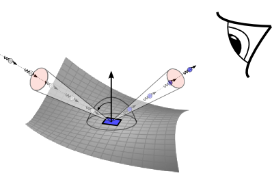
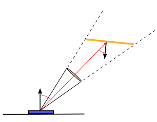
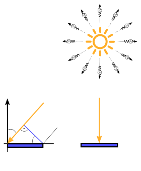
$L_o(\mathbf{v}) = L_e(\mathbf{v}) + \int\limits_\Omega \mathrm{f}_r(\mathbf{v}, \mathbf{l})\, \, \underbrace{L_i(\mathbf{l}) \cos(\theta) \, d\omega}_{dE(\mathbf{l})}$
struct RayPayloadType {
vec3 radiance;
vec3 nextRayOrigin;
vec3 nextRayDirection;
vec3 nextFactor;
int level;
}; // type of the "payload" variable
...
void main() { /**** RAY GENERATION SHADER ****/
// compute random pixel offset
vec2 pixelOffset = hammersley(uint(frameID), uint(frameSize));
// compute the texture coordinate for the output image in range [0.0, 1.0]
vec2 texCoord = (vec2(gl_LaunchIDEXT.xy) + pixelOffset) / vec2(gl_LaunchSizeEXT.xy);
// camera parameter
float aspect = float(gl_LaunchSizeEXT.x) / float(gl_LaunchSizeEXT.y);
vec3 rayOrigin = camPos;
vec3 rayDirection = getCameraRayLookAt(30.0, aspect, camPos, camLookAt, camUp, texCoord);
uint rayFlags = gl_RayFlagsNoneEXT; // no ray flags
float rayMin = 0.001; // minimum ray distance for a hit
float rayMax = 10000.0; // maximum ray distance for a hit
uint cullMask = 0xFFu; // no culling
// init ray and payload
payload.nextRayOrigin = rayOrigin;
payload.nextRayDirection = rayDirection;
payload.nextFactor = vec3(1.0);
vec3 contribution = vec3(1.0);
vec3 color = vec3(0.0, 0.0, 0.0);
int level = 0;
const int maxLevel = 5;
// shot rays
while(length(payload.nextRayDirection) > 0.1 &&
level < maxLevel && length(contribution) > 0.001) {
payload.level = level;
// Submitting the camera ray to the acceleration structure traversal.
// The last parameter is the index of the "payload" variable (always 0)
traceRayEXT(topLevelAS, rayFlags, cullMask, 0u, 0u, 0u,
payload.nextRayOrigin, rayMin, payload.nextRayDirection, rayMax, 0);
color += contribution * payload.radiance;
contribution *= payload.nextFactor;
level++;
}
if(frameID == 0) {
gsnSetPixel(vec4(color, 1.0));
} else {
vec3 previousAverage = gsnGetPreviousPixel().rgb;
previousAverage = pow(previousAverage, vec3(2.2)); // inverse gamma correction
vec3 newAverage = (previousAverage.rgb * float(frameID) + color) / float(frameID + 1);
newAverage = pow(newAverage, vec3(1.0 / 2.2)); // gamma correction
gsnSetPixel(vec4(newAverage, 1.0));
}
}
void main() { /**** CLOSEST-HIT SHADER ****/
// get mesh vertex data in object space
vec3 p0, p1, p2;
gsnGetPositions(gl_InstanceID, gl_PrimitiveID, p0, p1, p2);
vec3 n0, n1, n2;
gsnGetNormals(gl_InstanceID, gl_PrimitiveID, n0, n1, n2);
vec2 t0, t1, t2;
gsnGetTexCoords(gl_InstanceID, gl_PrimitiveID, t0, t1, t2);
// interpolate with barycentric coordinate
vec3 barys = vec3(1.0f - baryCoord.x - baryCoord.y, baryCoord.x, baryCoord.y);
vec3 localNormal = normalize(n0 * barys.x + n1 * barys.y + n2 * barys.z);
vec3 localPosition = p0 * barys.x + p1 * barys.y + p2 * barys.z;
vec2 texCoords = t0 * barys.x + t1 * barys.y + t2 * barys.z;
// transform to world space
mat3 normalMat;
gsnGetNormal3x3Matrix(gl_InstanceID, normalMat);
vec3 normal = normalize(normalMat * localNormal);
vec3 position = gl_ObjectToWorldEXT * vec4(localPosition, 1.0);
// assign materials
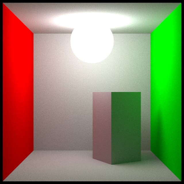
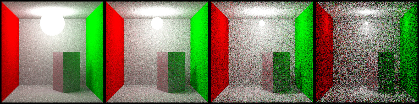
// Cornell Box
vec3 baseColor = cornellWhite;
vec3 emission = vec3(0.0);
if(gl_InstanceID == 2 && texCoords.x < 0.25) {
baseColor = cornellRed;
}
if(gl_InstanceID == 2 && texCoords.x >= 0.5 && texCoords.x < 0.75) {
baseColor = cornellGreen;
}
// light sphere
if(gl_InstanceID == 1) {
baseColor = vec3(0.0);
emission = vec3(20.0);
}
// different random value for each pixel, each level, and each frame
vec3 random = random_pcg3d(uvec3(gl_LaunchIDEXT.xy, frameID + payload.level));
// uniform sampling of hemisphere
float theta = 0.5 * PI * random.y;
float phi = 2.0 * PI * random.x;
payload.radiance = emission;
// sampled indirect diffuse direction in normal space
vec3 localDiffuseDir = vec3(sin(theta) * cos(phi), sin(theta) * sin(phi), cos(theta));
vec3 diffuseDir = getNormalSpace(normal) * localDiffuseDir;
payload.nextRayOrigin = position;
payload.nextRayDirection = diffuseDir;
payload.nextFactor = baseColor * PI * cos(theta) * sin(theta);
}
void main() { /**** MISS SHADER ****/
// set color to black
payload.radiance = vec3(0.0, 0.0, 0.0);
// no more reflections
payload.nextRayOrigin = vec3(0.0, 0.0, 0.0);
payload.nextRayDirection = vec3(0.0, 0.0, 0.0);
}

| PDF / Mapping | Top view | Side view |
|---|---|---|
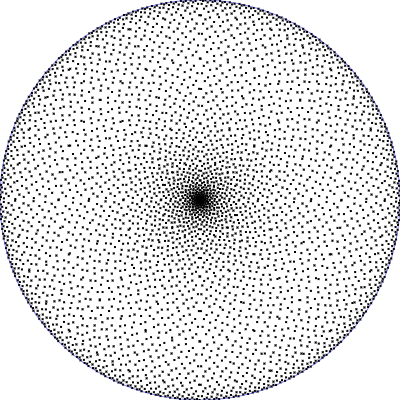
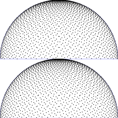
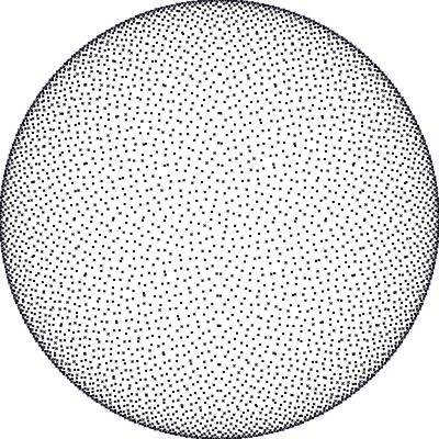
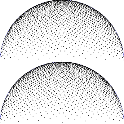
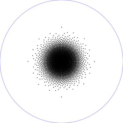
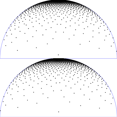
| Uniform sampling of polar angles
$\mathrm{p}(\theta, \phi) = \frac{1}{2\pi} \frac{1}{\pi/2}$
$\phi = 2 \pi \,u$
$\theta = \frac{\pi}{2}\, v$
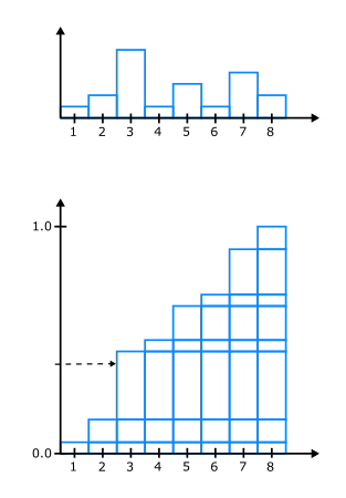
(corresponds to the Riemann sum)
|
|
|
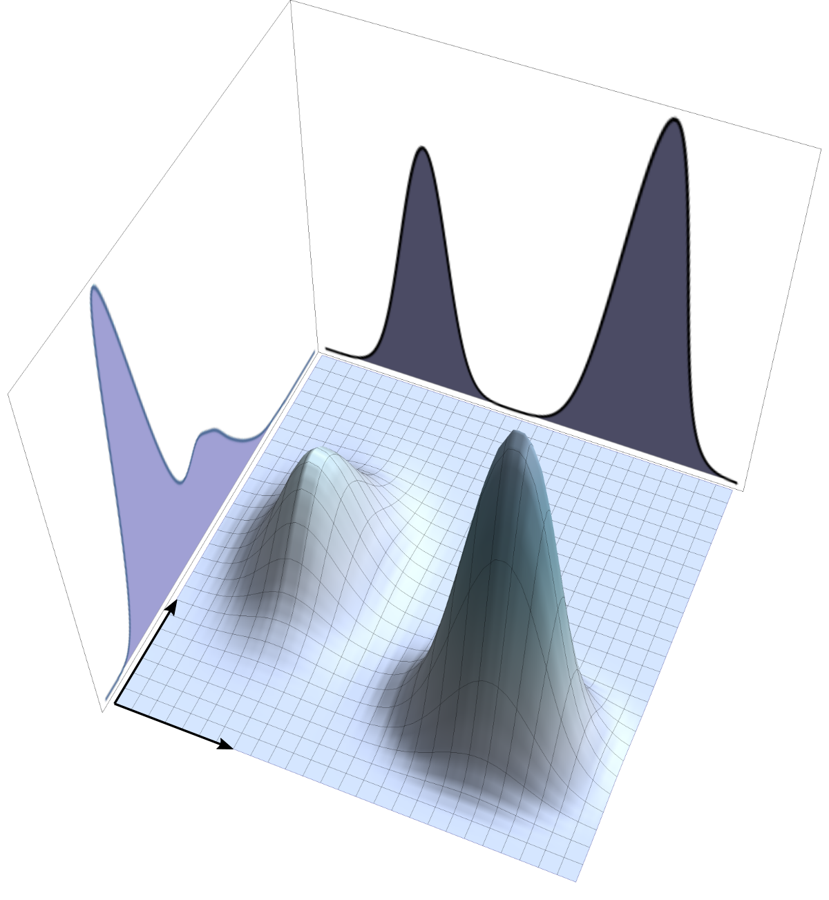
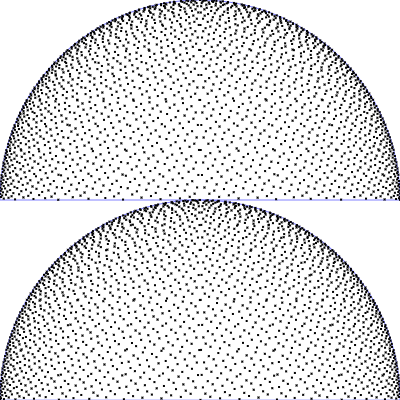
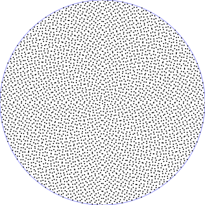
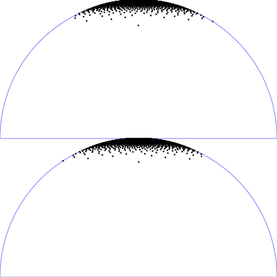
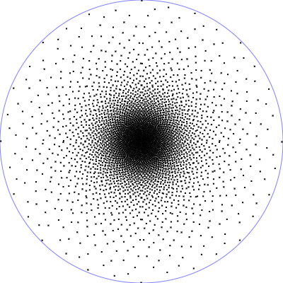
| Uniform sampling of a hemisphere
$\mathrm{p}(\theta, \phi) = \frac{1}{2\pi} \,\sin(\theta)$
$\phi = 2 \pi \,u$
$\theta = \arccos(1 - v)$
|
|
|
| PDF / Mapping | Top view | Side view |
|---|---|---|
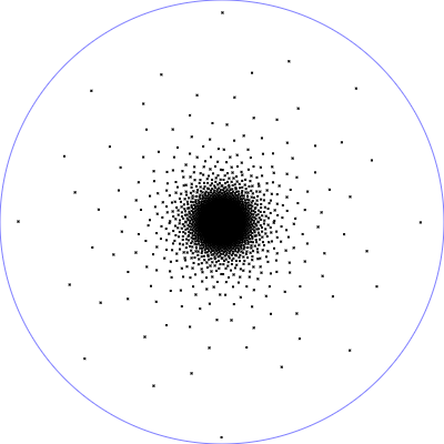
| Phong BRDF (diffuse part)
$\mathrm{p}(\theta, \phi) = \frac{1}{\pi} \, \cos(\theta) \,\sin(\theta)$
$\phi = 2 \pi \,u$
$\theta = \arcsin(\sqrt{v})$
|
|
|
| Phong BRDF (specualar part)
$\mathrm{p}(\theta, \phi) = \frac{n_s + 1}{2 \pi} \, \cos(\theta)^{n_s} \,\sin(\theta)$
$\phi = 2 \pi \,u$
$\theta = \arccos\left((1-v)^{\frac{1}{n_s+1}}\right)$
|
|
|
| PDF / Mapping | Top view | Side view |
|---|---|---|
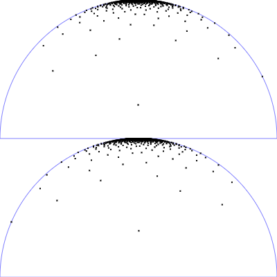
| Microfacet GGX distribution with $r_p = 0.5$ und $\alpha = r_p^2$
$\mathrm{D}_{\tiny \mbox{GGX}}(\theta) = \frac{\alpha^2}{\pi \left(\cos^2(\theta) (\alpha^2-1)+1\right)^2}$
$\mathrm{p}(\theta, \phi) = \mathrm{D}_{\tiny \mbox{GGX}}(\theta)\cos(\theta)\sin(\theta)$
$\phi = 2 \pi \,u$
$\theta = \arccos\left(\sqrt{\frac{1 - v}{v (\alpha^2-1) + 1} }\right)$
|
|
|
| Microfacet GGX distribution with $r_p = 0.25$ |
|
|

float theta = 0.5 * PI * random.y;
float phi = 2.0 * PI * random.x;
vec3 localDiffuseDir = vec3(sin(theta) * cos(phi), sin(theta) * sin(phi), cos(theta));
vec3 diffuseDir = getNormalSpace(normal) * localDiffuseDir;
payload.nextRayOrigin = position;
payload.nextRayDirection = diffuseDir;
payload.nextFactor = baseColor * PI * cos(theta) * sin(theta);
float theta = asin(sqrt(random.y));
float phi = 2.0 * PI * random.x;
vec3 localDiffuseDir = vec3(sin(theta) * cos(phi), sin(theta) * sin(phi), cos(theta));
vec3 diffuseDir = getNormalSpace(normal) * localDiffuseDir;
payload.nextRayOrigin = position;
payload.nextRayDirection = diffuseDir;
payload.nextFactor = baseColor;

Please notify me by e-mail if you have questions, suggestions for improvement, or found typos: Contact